®
THE D\TNAMilCS OF
KlflDHB
This page is intentionally left blank
®
THE DYNAMICS OF
PATTERNS MI Rabinovich University of California, San Diego
A B Ezersky Russian Academy of Sciences
P D Weidman University of Colorado
World Scientific Singapore • New Jersey • London • Hong Kong
Published by World Scientific Publishing Co. Pte. Ltd. P O Box 128, Farrer Road, Singapore 912805 USA office: Suite IB, 1060 Main Street, River Edge, NJ 07661 UK office: 57 Shelton Street, Covent Garden, London WC2H 9HE
British Library Cataloguing-in-Publication Data A catalogue record for this book is available from the British Library.
THE DYNAMICS OF PATTERNS Copyright © 2000 by World Scientific Publishing Co. Pte. Ltd. All rights reserved. This book or parts thereof, may not be reproduced in any form or by any means, electronic or mechanical, including photocopying, recording or any information storage and retrieval system now known or to be invented, without written permission from the Publisher.
For photocopying of material in this volume, please pay a copying fee through the Copyright Clearance Center, Inc., 222 Rosewood Drive, Danvers, MA 01923, USA. In this case permission to photocopy is not required from the publisher.
ISBN 981-02-4055-4 ISBN 981-02-4056-2 (pbk)
Printed in Singapore by FuIsland Offset Printing
To our parents,
Dora and Israel ovetlana ana Doris Ora ana Merle
This page is intentionally left blank
Preface
The creative process of writing this book was less a result of that which arises out of ones own head, hand, pen and paper than a result of the in teractive dialogue between authors with a similar vision. Our desire is to present a clear and concise presentation of principal phenomena, basic con cepts, and novel ideas in pattern formation using the language of nonlinear dynamics supplemented by photographs of actual patterns observed in the laboratory. We believe, perhaps a little presumptuously, that the principle we adhere to, namely "one chapter - one topic" together with a careful se lection of examples, has enabled us to write a book that is comprehensible to graduates, postgraduates, and those researchers who have just started investigating this extremely fascinating field of science. As is well known, the elegance of simplicity tempts one to simplify real phenomena by fitting them to conventional and universal models. We hope that we succeeded in avoiding this temptation unduly, since every chapter is focused on specific experiments. The text is supplemented with two appendices. Appendix A — A Short Guide to Nonlinear Dynamics — is provided as a review of the theoretical underpinnings of nonlinear systems and Appendix B — Key Experiments in Pattern Formation — is included for readers curious about experimental setups designed to observe pattern phenomena in the laboratory. For the most part, the book is based on the lectures read by MIR to students of the University of Nizhny Novgorod, the University of Chicago, and the University of California at San Diego. Some sections are the result of laboratory experiments spearheaded by ABE and PDW. We greatly appreciate numerous discussions on the topics presented vii
Vlll
Preface
herein with H. Abarbanel, V. Afraimovich, I. Aranson, A. Gaponov-Grekhov, L. Kadanov, J. Lebowitz, A. Libchaber, Ya. Sinai, L. Tsimring and P. Varona. The authors are indebted to F. Hjguera for a careful reading of Chapter 10 and to J. Meiss and B. Polotovsky for critical comments concering Appendix A. In addition, L. Tsimring wrote Chapter 11 upon request of the authors. We are ever indebted to Nadezhda Krivatkina and Leonid Rubchinsky who helped us prepare the manuscript, to Michael Sprague for suggestions to improve the layout, and to Kendall Hunter for rescuing files sent to Boulder from Nizhny Novgord. MIR acknowledges support from the En gineering Research Program of the Office of Basic Energy Science at the Department of Energy and personally Robert Price who is deeply interested in the subjects discussed in this book. We also appreciate the support of International Center for Advanced Studies in Nizhny Novgorod.
M. I. Rabinovich A. B. Ezersky P. D. Weidman Boulder, Colorado August 2000
Contents
Preface
vii
Chapter 1
Patterns: Prelude to a Dynamical Description
Chapter 2
Linear Stage of Pattern Formation
1 15
Chapter 3 Model Equations 3.1 Swift-Hohenberg equation 3.2 Newell-Whitehead-Segel equation 3.3 Coupled amplitude equations 3.4 Phase equations
27 29 35 38 42
Chapter 4 The Ginzburg-Landau Equation 4.1 The dissipative Ginzburg-Landau equation 4.2 Nerve membrane excitation and the CGL equation 4.3 Optical dynamics and the CGL equation 4.4 Simple patterns in the CGL equation 4.5 Phase equations revisited 4.6 Gallery of phenomena
45 46 48 50 52 55 57
Chapter 5
63
'Crystal' Formation
Chapter 6 Quasicrystals 6.1 Octagons, decagons, and dodecagons 6.2 A generalized Swift-Hohenberg model 6.3 The 'turbulent' crystal ix
75 78 81 82
x
Contents
Chapter 7 Breaking of Order 7.1 A simple model for domain walls 7.2 Topological defects 7.3 The birth of penta-hepta defects 7.4 Dislocations and domain walls in Faraday ripples
87 89 92 96 102
Chapter 8 Localized Patterns 8.1 Bistable media 8.2 Dynamical disorder of structures 8.3 Particle interaction 8.4 Chaotic scattering
107 107 114 115 118
Chapter 9 Spirals 9.1 Active spirals 9.1.1 Spirals in 9.1.2 Spirals in 9.2 Passive spirals 9.2.1 Spirals in 9.2.2 Spirals in
129 133 the complex Ginzburg-Landau equation . . . 133 the FitzHugh-Nagumo model 136 142 the Faraday experiment 143 Rayleigh-Benard convection 145
Chapter 10 Patterns in Oscillating Soap Films 10.1 Introduction 10.2 Observations 10.3 Models for vorticity generation 10.3.1 Marangoni wave model 10.3.2 The role of air
151 151 152 158 160 162
Chapter 11 Patterns in Colonies of Microorganisms 11.1 Dictyostelium discoideum 11.2 Esherichia coli 11.3 Bacillus subtilis
173 174 178 184
Chapter 12 Spatial Disorder 12.1 Introductory remarks 12.2 Characteristics of space series 12.3 The Grassberger-Procaccia algorithm 12.4 Qualitative description of developing disorder 12.5 Dynamical dimension of defect-mediated turbulence
189 189 193 197 199 202
Contents
xi
Chapter 13 Patterns in Chaotic Media 13.1 Introductory remarks 13.2 Chaotic synchronization 13.3 Coexistence of regular patterns and chaos 13.4 Coarse grain spatio-temporal patterns 13.5 Coherent patterns on a chaotic checkerboard
205 205 208 211 214 220
Chapter 14 Epilogue: Living matter and dynamic forms 14.1 Hallucinations 14.2 Spatio-temporal patterns and information processing
225 227 234
Appendix A A Short Guide to Nonlinear Dynamics A.l Dynamical systems A.1.1 Types of dynamical systems A.1.2 Equilibrium states A. 1.3 Homoclinic and heteroclinic trajectories A.1.4 Limit cycles A. 1.5 Quasiperiodic motion A.2 Bifurcations A.2.1 Bifurcations of equilibrium states A.2.2 Birth of periodic motions A.2.3 Change of stability in periodic motions A.3 Chaotic Oscillations A.3.1 Characteristics of chaos and the strange attractor A.3.2 Chaotic Hamiltonian systems A.3.3 Chaotic self-excited oscillations A.4 Synchronization of oscillations A.5 Dynamical chaos and turbulence
239 239 240 241 245 248 249 250 252 258 260 261 261 263 264 266 271
Appendix B Key Experiments in Pattern Formation B.l Parametrically excited patterns B.l.l Experiments with liquids B.1.2 Experiments with granular material B.2 Thermal convection B.2.1 Rayleigh-Benard convection B.2.2 Patterns in Rayleigh-Benard convection B.2.3 Benard-Marangoni convection B.3 Diffusive chemical reactions
...
279 279 279 287 292 292 295 297 302
xii
Contents
B.3.1 Turing patterns
302
B.3.2
306
Oscillating chemical reactions
Bibliography
309
Index
320
Chapter 1
Patterns: Prelude to a Dynamical Description
The theory has to be as simple as possible but not simpler. Albert Einstein The diversity of patterns existing in the surrounding world usually arouses amazement not only in fiction novels but in scientific literature also. Perhaps still more curious is the fact that these diversified patterns are universal to a certain extent: hexagonal patterns on a giraffe's skin and hexagonal structures emerging at the onset of convection in a liquid layer; isolated patterns in colonies of microorganisms and soliton structures in hydrodynamics and in nonlinear optics; spiral chaos in heart muscle fibril lation and spiral turbulence in chemical systems; and a multitude of other examples. What is the nature of this universality? Why do analogous spatial pat terns arise in systems that are so different? Answers to these questions can be found using key results gleaned from the classical theory of oscil lations. It suffices here to recall that the type of oscillations — periodic, quasiperiodic, chaotic, harmonic, or relaxational — is determined by the dynamical properties of the system (e.g. the number of degrees of freedom, the type of nonlinearity, and the presence of fast and slow motions) inde pendent of whether the system is acoustical, optical, hydrodynamical, or chemical. An analogous situation exists for the birth and development of spatial patterns. It might seem at first sight that an infinite diversity of such patterns makes their unified dynamical description a hopeless, even meaningless task. However, here again one can exploit the knowledge ac cumulated in the classical theory of oscillations, in particular the ideas put forth by Andronov in 1931 concerning the structural stability of dynamical l
2
Patterns:
Prelude to a Dynamical
Description
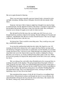
systems and the investigation of their bifurcations. We briefly review the es sential points of these ideas, the roots of which are traced back to Poincare. In his book La Valeur de la Science in the chapter entitled Analysis and Physics, Poincare (1905) wrote that "The main thing for us to do with the equations of mathematical physics is to investigate what may and should be changed in them." Indeed, any description of real life is a model, and in modeling the dynamics of nonlinear systems one is usually confronted with ordinary or partial differential equations containing different nonlinear dependencies. Ideally it would be great to obtain their general solutions and thus predict the behavior of a given model subject to specific initial conditions. However, it is only by rare luck that one is able to find all integrals of a nonlinear system of differential equations. Andronov's remarkable approach toward understanding such systems contained three key points: (i) Only those models demonstrating motions which do not vary with small changes of the parameters can be regarded as really interesting ones — Andronov referred to these as models or dy namical systems that arc structurally stable; (ii) To obtain insight into the dynamics of a system means to clarify all principal types of its behavior under all possible initial conditions, i.e. one should investigate the behav ior of the model as a whole rather than find particular solutions under specific initial conditions — hence Andronov's fondness of the methods of phase space analysis; and, finally, (iii) Consideration of the behavior of the system as a whole allows one to introduce the concept of topological equiv alency of dynamical systems, and requires an understanding of local and global bifurcations as control parameters are varied. Conservation of the topology of the phase portrait corresponds to a qualitatively stable motion of the system with small variation of governing parameters. Partitioning of the space of parameters into regions with different behavior then furnishes a complete picture of the potentialities of a dynamical model (Andronov et ai, 1973a, 1973b). Under certain idealizations it is natural to consider the process of pat tern formation as the life of a dynamical system. The features of this life as t —> oo then determine the characteristic aspects of the spatial patterns, be they perfect or irregular. Let us consider the experimental results reproduced here in Figures. 1.1, 1.2 and 1.3 taken from three different investigations of patterns formed on the surface of a liquid. Figure 1.1 is a photograph of a regularly rough free surface of progressive water waves a channel; Fig. 1.2 exhibits a hexagonal
Patterns:
Prelude to a Dynamical
Description
3
Fig. 1.1 Spilling breaking waves on a water surface; the waves propagate from left to right. Taken from (van Dyke, 1982).
lattice of Rayleigh-Benard convection (see Appendix B.2); and Fig. 1.3 displays an irregular pattern of capillary ripples formed on a liquid layer contained in a vertically vibrating cavity (this so-called Faraday experiment is discussed in Appendix B.l). In viewing these patterns many questions arise: Why are the patterns steady? How are they formed out of arbitrary initial conditions? In what way does the pattern change with the variation of experimental parameters? How is one able to describe the patterns? The latter question seems to be simpler than the others and we therefore take it as a starting point in the construction of a dynamical theory of space patterns. The first observation that catches the eye is the existence of a definite spatial scale. It is the characteristic length describing the spanwise and streamwise extent of the propagating wave system in Fig. 1.1 and in Fig. 1.2 it is the well-defined hexagonal scale of instability. Thus it seems natural to suppose that the observed spatial field can be represented as a su perposition of plane waves having wavenumber vectors of equal magnitude, viz. u(r,0 = 5Ian(«)eik"r+c.c.
(1-1)
n
where the coefficients an(t) are scalar quantities and all wave vectors k n satisfy |k n | = ko. Then, four modes having wave vectors at right angles to one another as in Fig. 1.4a correspond to a lattice with square cells, and six plane waves with wave vectors forming an angle of 60° with one another as
4
Patterns:
Prelude to a Dynamical
Description
Fig. 1.2 Shadowgraph image of hexagonal cells obtained in Rayleigh-Benard convection in a thin horizontal layer of CO2 under pressure. Taken from (Bodenschatz et al., 1991).
in Fig. 1.4b correspond to a lattice of hexagonal cells. The capillary pattern shown in Fig. 1.3 may be formed by superposing a sufficient number of spatial modes with wave vectors of equal magnitude, provided they are randomly distributed in angle as in Fig. 1.4c. The com puter image of a simple random mode distribution in Fig. 1.5 goes a long way toward mimicing the actual experimental snapshot of Fig. 1.3. There exist, between the limiting purely periodic and irregular field distributions in space, numerous intermediate patterns having different de grees of irregularity (or order). One of the most remarkable achievements obtained in recent years is the discovery of quasicrystal order in hydrodynamic flows which appears, for example, in capillary ripples parametrically excited by an oscillating gravitational field (Christiansen et al., 1992; Ed wards and Fauve, 1993); see Chapter 6 for theoretical details. Typical quasicrystal patterns are presented in Figs. 1.6 and 1.7. Computer simulations readily reproduce these quasiperiodic patterns for which long-range order is typical by incorporating eight (Fig. 1.8a) or twelve (Fig. 1.8b) plane waves of equal wave vector magnitude forming, respectively, angles of 45° and 30° with one another. However, the fact
Patterns:
Fig. 1.3 1986).
Prelude to a Dynamical
Description
5
Chaotic pattern of free surface capillary ripples. Taken from (Rzersky et al.,
K
*>• ***
,y-~~
V Ky'"
/S 5?\. ^]'~ \y " --..
a
b
v
c
Fig. 1.4 Wavenumber vectors |k|„ = ko of spatial modes forming (a) a square pattern, (b) a hexagonal pattern, and (c) a disordered pattern.
that a quasicrystal may be constructed using only eight (or twelve, or n) modes does not explain the existence of the patterns observed. Indeed, why are eight (or twelve) modes persistently encountered? What, generally, determines their number? Is it possible to change the type of quasicrystal symmetry by changing the parameters as, for instance, the frequency of an oscillatory gravitational field or the depth of the fluid layer? Here, again, a dynamical theory is needed to resolve these questions. Figure 1.9 shows the evolution of Benard-Marangoni convection from
6
Patterns:
Prelude to a Dynamical
Description
Fig. 1.5 Computer simulation of a disordered pattern with a spatial spectrum like that in Fig. 1.4c. Taken from (Blumel et al., 1992).
Fig. 1.6 Eight-fold quasicrystal pattern on a liquid layer driven by harmonic vertical forcing. The image of ripples is formed by light reflected from the free surface. Taken from (Christiansen el al., 1992).
a random initial state in a laboratory experiment. It is clear that the field becomes more ordered with time. For this situation the principal questions to ask of the dynamical theory are: What kind of structure will be established as t -> oo? Will it be a regular hexagonal lattice or will it have some disorder in the form of defects? If the latter, how will the defects evolve in time? Of what must a dynamical theory of patterns consist? The principal ob jectives of such a theory are: (i) an analysis of the hierarchy of instabilities and the birth of various patterns in the course of evolution from an ini tial state, (ii) an investigation of the mutual transformation of patterns as control parameters are varied, (iii) an analysis of possible hysteretic effects
Patterns:
Prelude to a Dynamical
Description
7
Fig. 1.7 Twelve-fold quasicrystal pattern on a liquid layer driven by biharmonic external forcing; experiments in (a) a circular cell and (b) a cell with boundary in the shape of France. Taken from (Edwards and Fauve, 1993).
Fig. 1.8 Wavenumber vectors of spatial modes forming (a) eight-fold and (b)twelve-fold quasicrystals.
in the system, and (iv) an investigation of differences between hand-made spatial chaos (see, for example, the painting by Pollack in Fig. 1.10) and dy namical chaos. Much can be done in this direction employing a traditional mode description of nonlinear fields, i.e. replacing the governing PDE's by their finite-dimensional ODE models. In this manner dynamical systems appear in a very natural fashion: for example, the time-dependent mode amplitudes an(t) in Eq. (1.1) may be described by ODE's. Many results of the classical theory of dynamical systems can be used directly if, and when, an appropriate physical meaning may be attached to the variables in the
8
Patterns: Prelude to a Dynamical Description
Fig. 1.9 Snapshots of B6nard-Marangoni convection at three successive times: (a) t = to, (b) t = t\ > to and (c) t = ti >t\. Taken from (Gaponov-Grekhov and Rabinovich, 1990).
Fig. 1.10 Oil on canvas painting entitled "Lavender Mist: Number 1" by Jackson Pol lock (1950); National Gallery of Art, Washington, DC.
model equations. Another important aspect of the theory to be developed is associated with the notion of a spatial dynamical system where one (or more) spatial coordinates play the role of time. A simple example is given by RayleighBenard convection which stably manifests ordered patterns that contain domains of rolls having different orientations. Such a pattern is depicted in Fig. 1.11. These types of problems will be considered in Chapter 12.
Patterns:
Prelude to a Dynamical Description
9
Fig. 1.11 Domain rolls observed in Rayleigh-B^nard convection in a circular cavity. Taken from (Ahlers et al., 1985).
Fig. 1.12
Domain wall numerically computed from Eqs. (1.2).
Here we just note that in special cases where a two-dimensional system can be transformed into a one-dimensional problem with spatial variable x, domains of uniform rolls are associated, as x -> +00 and x —► —00, with different equilibrium states of the spatial dynamical system. Moreover, an isolated trajectory (separatrix) connecting these equilibrium states cor responds to a boundary between domains, a so-called domain wall. This one-dimensional spatial dynamical system can be described by the following
10
Patterns:
Prelude to a Dynamical
Description
Fig. 1.13 A quasistable bound state of dislocations: a domain wall in parametrically excited ripples. Circles mark dislocations that propagate down to form the inclined domain wall. Taken from (Ezersky et ai, 1995).
pair of amplitude equations
^
= A.-lAl + pADA,
££■
=
A2-[Al + pAl]A2
(1.2)
in which A\(x) and A2(x) are the amplitudes of the modes forming the pattern and p > 1 is the coefficient of mode competition (see Chapter 7 for details). Separatrices of the dynamical system (1.2) meeting the condition Ai(+oo) = 1, A2(+oo) = 0 and A\(—00) = 0, A2{—00) = 1 correspond to a jump in mode amplitude across the domain wall. The pattern described by Eqs. (1.2) exhibits a domain wall like that displayed in Fig. 1.12. When the roll axes are slightly inclined with one another, a pattern like that in Fig. 1.13 is formed (Ezersky et ai, 1995). Circles in this figure mark individual dislocations that evolve in a chain-like fashion to form the inclined domain wall observed in the figure. If several different modes coexist, their nonlinear interaction is likely
Patterns:
Prelude to a Dynamical
Description
11
Fig. 1.14 Pattern in Rayleigh-Benard convection in a layer of CO2 under pressure at a Prandtl number near one. Taken from (Morris et al., 1993).
to produce an irregular or chaotic solution of a spatial dynamical system. This is the simplest example of deterministic disorder to which an invari ant chaotic set corresponds in phase space. Field distributions (of velocity, temperature, concentration, etc.) are called order parameters. In the next level of disorder, singularities of the order parameters can exist giving rise to more complicated dynamical patterns such as that shown in Fig. 1.14 for Rayleigh-Benard convection at Prandtl numbers near unity. This is an example of the recently discovered spatial disorder known as spiral-defect chaos; see, for example, (Morris et al., 1993). It consists of a disordered pattern of convection rolls featuring the spontaneous appearance and dis appearance of rotating spiral defects. One feature of spiral defects that differentiates them from defects in many other systems is that they are not constrained to be created in pairs. The spiral-defect state behaves as an individual element comprised of single spirals with clockwise or counter clockwise winding. The mechanics for the creation of this variety of forms is not yet completely understood, but numerical simulations show that a crucial element for the formation of such patterns and individual spirals is the strength of the mean-drift field. Further and more detailed discussion of spiral defects will be given in Chapter 9. How may disordered patterns be understood? When discussing the con cept of disorder even physicists have quite different associations. Experts
12
Patterns:
Prelude to a Dynamical
Description
in statistical physics think of the disordered arrangement of molecules in a gas or liquid at an arbitrary moment of time, whilst solid-state physicists envisage the disorder of magnetic domains and spin orientation. Gener ally speaking, disorder is a complex, irregular spatial distribution of some elements or fields. Traditional characteristics of disorder are closely con nected with the determination of correlation lengths. For instance, when concerned with long-range order we have in mind a situation where the dis tribution of a certain physical quantity (order parameter) in a given region of space is unambiguously related to its value at an infinitely distant region. Perhaps the most familiar example is long-range order in crystalline mate rials where a density correlation exists. A well known case for which only short-range order is possible is in the structure liquids; here the random motion of atoms gives rise to density fluctuations that destroy any possible long-range order. However, it has been relatively recently discovered that long-range crystal order does exist in hydrodynamics, a branch of physics in which crystal-like structures are not traditionally contemplated. This topic will be discussed in Chapters 5 and 6. The dynamical theory of disorder describes irregular spatial field distri butions, such as the electron density distribution in crystals or the density distribution of matter in galaxies, employing methods of nonlinear dynam ics. We are trying to understand whether spatially irregular distributions of physically meaningful fields may have a dynamical origin. In other words, might there exist irregular field distributions that can be described by dy namical models? It is anticipated that if the fields have physical origin, they will be described by partial differential equations or some more spe cific equations for dynamical systems with several 'times,' where the spatial coordinates represent the 'times.' Even the simplest spatio-temporal analogy convinces us that finitedimensional disorder — an irregular spatial field distribution described by a dynamical system possessing a finite number of degrees of freedom — must exist in Nature and must be no less prevalent than finite-dimensional tem poral chaos. There are plenty of examples such as stationary chaotic waves observed in different physical systems. There arises a natural impulse to apply results of the theory of temporal dynamical chaos to problems involv ing spatial dynamical disorder. The application is trivial to a certain extent if we have one spatial coordinate and a steady regime. However, very diffi cult problems arise even for systems described by a single spatial coordinate. The main question is: Does spatially disordered initial data in that system
Patterns:
Prelude to a Dynamical
Description
13
evolve deterministically in time? When we consider two-dimensional (and especially three-dimensional) spatial disorder of a dynamical origin, quali tatively new problems arise. The commensurability-quasiperiodicity-chaos transition (see Appendix A.5) is well known in simple dynamical systems involving low-dimensional ordinary differential equations. By replacing the time variable with a single space coordinate, we can expect to find the same transition scenario for spatial disorder in one-dimensional media. Is such a sequence possible through the variation of a governing parameter for a twoor three-dimensional field? What kind of dynamical system will describe such disorder? We have no definite answer to these questions yet. However, the classical commensurability-quasiperiodicity-chaos transition scenario is highly probable. Returning to the mode superposition description of disorder, it is per haps not so surprising that a randomly disordered field like the one shown in Fig. 1.3 may be described by the superposition of a large number of harmonic waves of equal wavelengths. Indeed, what else could be expected if the mode amplitudes are random, their phases are arbitrary, and the wave vector orientations are also random as in Fig. 1.4c? Note that space correlations of a Gaussian amplitude distribution u(r) decay rather fast in accord with the following formula found by (Berry, 1983) K(X) = Ju(T)u(r
+ X)d2r
~ J0(k0\x\)
(1-3)
in which Jo is the Bessel function of order zero, k0 is the wave vector modulus, and x ls the argument of the correlation function. The close similarity between the computer imaging of random mode superposition in Fig. 1.5 with the snapshot of the distribution of capillary waves in Fig. 1.3 produces a very important question: Why have the wave amplitudes estab lished a Gaussian distribution with arbitrary phases not synchronized in time? These facts must be accounted for by any realistic dynamical theory.
Chapter 2
Linear Stage of Pattern Formation
Prediction is difficult, especially if it concerns the future. An old Chinese proverb How does an initial, absolutely symmetric (homogeneous) state of a medium or field become inhomogeneous? This usually results from a spon taneous breaking of symmetry which represents the change of stability of a stationary state. Symmetry breakings (c/. Appendix A.2) are frequently observed, sometimes without realizing it. Consider making coffee directly from a uniform horizontal layer of granulated coffee beans floating on the surface of water in a broad saucepan. What will be observed? The layer of steam that facilitates extraction of the coffee rises from the bottom of the vessel and disintegrates into individual bubbles thereby producing a coffee surface in the form of hills and valleys. If we remove the saucepan from the stove before it comes to a boil, the coffee particles that have slipped down to the valleys will 'remember' this inhomogeneous state which corre sponds to a spontaneous breaking of spatial symmetry. Such a transition occurs monotonically in time and is often referred to as a Turing bifurca tion (Turing, 1952) or an exchange of stability (Davis, 1969), unlike the Andronov-Hopf bifurcation which corresponds to a transition to an oscilla tory instability (see Appendix A). Turing revealed this exchange of stability in chemical reactions with diffusion nearly a half century ago and was the first to establish a connection between the spontaneous birth of inhomoge neous patterns with the mechanism of morphogenesis in biology. See, for instance, the nice review by (Koch and Meinhardt, 1994) where one can find many interesting examples of Turing patterns in biology. Turing showed that under certain conditions even just two interacting chemicals can gen15
16
Linear Stage of Pattern Formation
erate stable inhomogeneous nonoscillatory patterns if one of the substances diffuses much faster than the other. This result is not at all intuitive since diffusion is expected to smooth out concentration differences rather than produce them. The exchange of stability bifurcation may be investigated using the diffusion reaction equations
|=f(u,«+DV2u
(2.1)
where u is the population vector, f (u, /?) determines the point reaction ki netics with control parameter /3, and D is the diffusion matrix. A standard linear stability analysis for a uniform density distribution, u = uo, with respect to spatial perturbations of wavenumber k in the form e'(k'""', gives a complex dispersion relation from which the Lyapunov exponent A(k,/3) and frequency w(k, /?) are determined. The critical wavenumber k c corre sponding to the minimum value of the control parameter pc at which the growth rate a = Re(A) first becomes positive may also be determined from this dispersion equation. The characteristic feature of the Turing instability corresponding to the class of space-symmetry-breaking instabilities is that A is real, i.e. u = Im(A) = 0; thus there are no temporal oscillations at the onset of instability. Owing to the symmetry properties of Eq. (2.1), which represent the properties of homogeneity and isotropy of the solution in which the chemical reaction occurs, the instability rate a depends only on the magnitude fco of wavenumber k and not on its direction. In other words, the linear stage of spontaneous symmetry breaking simply increases the field strength which, in general, may be represented in the form /•2JT
[A^e^-T
u(r, t) = uo+
+ A^e~ik*-r] dip
(2.2)
Jo in which Av and kv are the amplitude and wavenumber distributions for waves propagating in the direction 8 = tp and |ky,| = ko. Of course, the kind of spatial pattern realized as t —¥ oo may be determined only by application of some nonlinear theory. A simple example that demonstrates the onset of an inhomogeneous density distribution in the absence of temporal oscillations is the Brussela-
Linear Stage of Pattern
Formation
17
tor model (GlansdorfF and Prigogine, 1971) — = a + u2v - (1 + 0)u + at
DuV2u
-^-=0u-u2v + DvV2u. (2.3) at These equations describe the spatio-temporal dynamics of the intermediate components u and v in an autocatalytic chemical reaction with respective diffusion coefficients £>u and Dv. The reactions a —y u 2u + v -^> 3u
u-^c
(2.4)
describe the concentration of the original substances a and /3 for which the final products c and d are constant when all reaction rates 9?j equal unity. Setting the left-hand sides of Eqs. (2.3) to zero gives the uniform steadystate solution: u 0 = a, vo = 0/a- Inserting then u = a + u and v = - +v in Eqs. (2.3), and linearizing for small perturbations u and v, yields the pair of disturbance equations d_ dt where the linearized operator L is . L =
( P - 1 + DUV2 ( -0
-a
2
a2 \ + DvV2)-
(2 6)
-
Stability of the trivial solution u = v = 0 of Eq. (2.5) is determined by solv ing for the eigenvalues A„ corresponding to the eigenfunctions (un,vn) = (U„, V„)e*k"'r of L, since arbitrary perturbations can be written in the form
($)-E^'(t)If for some k„ one finds Re(A„) > 0 then the steady-state solution is unstable. Suppose for simplicity that u and v depend on the single space
Linear Stage of Pattern
Formation
Im A.
ImX
Re A
Fig. 2.1 Qualitative features of the eigenvalue A of Eq. (2.8) in (p,q) parameter space; the parabolic curve is q = ^ p 2 .
coordinate x in which case (iii,i)i) = (U\, Vi)elkx. Eq. (2.5) yields the characteristic equation for A
Then substitution into
A2 + pX + q = 0
(2.8)
where the coefficients p and q are given by p=a2
+ l-0
+ (Du + Dv)k2
q = a20 - (/? - 1 - k2Du)(a2
+
k2Dv).
(2.9)
The variation of Re(A) and Im(A) in (p, q) parameter space is shown in Fig. 2.1. The complex eigenvalue A has a positive real part if either of the coefficients p or q is negative. We are interested in the nonoscillatory instability which leads to a new steady-state structure, realized when q < 0 or when \p\ < -2y/q for q > 0. The homogeneous state is stable for ft < 1. For /? > 1, on the other hand, it is unstable either to temporal disturbances where the eigenvalue exhibits a pair of complex conjugate roots, or to monotonically growing disturbances when one root appears on the positive real axis of the Aplane. The Turing spontaneous exchange of stability, which requires 0 > 1, occurs when Du
Linear Stage of Pattern
Formation
19
P
Pmm
ko
k
Fig. 2.2 Neutral curve of the Turing instability for the Brusselator described by Eqs. (2.3).
The neutral stability boundary q(l3,k) = 0 depicted in Fig. 2.2 has the minimum value 0min and corresponding critical wavenumber k0 given by A™ = [l + a^/DJD^
,
kQ = y/a/y/DuDv.
(2.10)
The fact that a continuous spectrum of modes e , k r , having arbitrary orientation of wave vectors k, appears at infinitesimally small increments above the instability threshold fim)n enables one to observe various patterns in a stationary regime. They may be crystals, quasicrystals, disorder (like in Fig. 1.5), or partially ordered patterns like the ones observed by Swinney and collaborators in a large chemical membrane reactor (Vigil et al., 1992) reproduced here in Fig. 2.3. Another example is the evolving hexagonal pattern shown in Fig. 2.4 that appears via a gravitational instability when a heavy liquid layer lies above an immiscible liquid of lower density. Spatial instabilities in unbounded nonequilibrium media may have dif ferent physical origins. In dissipative media, as a rule, it is connected with the competition between forces which either facilitate or inhibit the development of instability. For example, the birth of patterns with char acteristic length scale A in Rayleigh-Benard convection in a liquid layer of thickness d heated from below stems from a competition between stabiliz ing viscous and thermal diffusion forces and destabilizing buoyancy forces
20
Linear Stage of Pattern Formation
Fig. 2.3 Partially ordered patterns in a large chemical gel reactor. The reactor consists of a thin (0.27 mm) disk-shaped layer of polyvinyl alcohol gel with one face in contact with a well-stirred chlorite-iodide-malonic reactant system and the other face in contact with transparent plexiglass. Taken from (Vigil et al., 1992).
Fig. 2.4 Development of Rayleigh-Taylor instability formed by inverting a thin layer (0.2 mm) of silicone oil spread across a flat glass plate; the view is looking down through the glass plate. Taken from (Fermigier et al., 1992).
(see Appendix B.2 for a detailed discussion of this system). The growth of a small perturbation giving rise to stable cellular convection is illustrated in Figs. 2.5 and 2.6; see also (Gershuni and Zhukhovitskii, 1976). Thermal diffusion and viscous damping are associated primarily with horizontal gra dients in the temperature and velocity fields at small wavelengths A < 2d like that sketched in Fig. 2.5; at large wavelengths A > 2d as in Fig. 2.6, on the other hand, viscous damping is primarily due to vertical gradients of those fields. The important control parameter for this flow is the Rayleigh number Ra = agATdP/nv, where a = (l/p)(dp/dT) is the thermal expansion coef-
Linear Stage of Pattern Formation
Z^
'/////////////<
21
////////
////////////////////////// Fig. 2.5 Sketch of the horizontal variation of temperature and velocity at mid-cell height in Rayleigh-B6nard convection for wavelengths A < 2d.
////////////?//////////////?////////////' Fig. 2.6
The same as Fig. 2.5, but for wavelengths A > 2d.
ficient, g is the acceleration due to gravity, p is the average fluid density, A T is the temperature difference between the warm bottom plate and the cooler top plate, and v and K are, respectively, the viscous and thermal diffusion coefficients of the fluid. The neutral stability curve Ra(k) for the classic Rayleigh-Benard system is plotted in Fig. 2.7. When Ra > Rac = 1708 stabilizing viscous and thermal diffusive forces are minimal and cellular convection spontaneously appears in the gap (Drazin and Reid, 1981). The critical dimensionless wavenumber kcd = 3.12 depicted in Fig. 2.7 corre sponds to an instability wavelength Ac = 2n/kc ~ 2d. A similar competition may be observed in other cases of spontaneous symmetry breaking, such as the development of Rayleigh-Taylor instability in a thin layer of heavy liquid overlaying a gas (or other lighter liquid) as illustrated in Fig. 2.8. This example exhibits a remarkable diversity of nontrivial two-dimensional patterns (Fermigier et al., 1992), so we shall consider it in some detail. Clearly, a thin layer of viscous fluid of uniform depth £o 'spread over a ceiling' will be unstable when subjected to the
Linear Stage of Pattern Formation
22
Ra ,,
2000
Ra.
1000
0
1
2
3
4
5
kd
Fig. 2.7 Neutral stability curve for Rayleigh-B6nard convection. Region I can be asso ciated with Fig. 2.6 and Region II with Fig. 2.5.
Fig. 2.8 System of coordinates for Rayleigh-Taylor instability of a liquid layer under a ceiling.
uniform gravitational field g = gez with unit vector e 2 pointing downwards as in Fig. 2.8. The time-dependent depth £ of the unstable layer will vary with the horizontal coordinates r = (x,y) so that
*(r,0=& + C(r,0
(2.11)
where £o is the undisturbed liquid depth. Assuming the liquid to be highly viscous, we neglect inertia effects and write the governing incompressible
Linear Stage of Pattern
Formation
23
Navier-Stokes equations in the form
vwg]=vP d2w dp p I Vw + 2 dz = dz~P9 _ dw V - u + — = 0. az
(2.12)
Here, p is the fluid density, p. = pv is the absolute fluid viscosity, u = (u, v) and w are respectively the horizontal and vertical components of the velocity field, p is the pressure, and the operators V 2 and V refer only to the horizontal coordinates x and y. The kinematic and dynamic boundary conditions are written as u = 0| i = o,
<9u
„
(2.13) *=«(<-,<)
Pa - P = 7 V • { V £ [1 + | V £ | 2 ] " 1 / 2 } ~ 7 V 2 e U=€(r,«)
(2-14)
where 7 is the coefficient of surface tension and pa is the constant atmo spheric pressure below the liquid layer. As for any thin layer (Phillips, 1977), the equations of motion may be written in the characteristic conser vation form
i+v-jf"*-0-
(2.15)
Taking into account the boundary conditions, Eq. (2.15) gives the evolution equation for the order parameter C,{r,t) (Fermigier et ai, 1992)
=
I ~f
{P9VH+7V C)
V [(3C+3C +e)V{p9
" ~f '
'
(2.16) when corrections of order (C/A) 2 are neglected, in which A is the charac teristic horizontal scale of the patterns. It follows from the form of the linear operator that the growth of C(r, t) is determined by the competition between the destabilizing force of gravity and the restoring force of surface tension. Growth of perturbations in the fluid depth vary with wavenumber
24
Linear Stage of Pattern Formation
Fig. 2.9 Instability growth rate as a function of wavenumber showing the competition between gravitationally dominant (fc < fco) and surface tension dominant (fc > fco) forces.
Fig. 2.10 Late time evolution of the Rayleigh-Taylor instability given in Fig. 2.4; this oblique view from below shows a regular array of pendant silicone oil drops hanging off the glass plate. Courtesy of Marc Fermigier.
according to the relation a(k) =
^(pgk2
7 fc
4
)
(2.17)
from which one finds at ko = \/pg/2j the maximum growth rate am = Qp2g2/l2fx-y as sketched in Fig. 2.9. Here again, as in Rayleigh-Benard convection, the orientation of the wave vector is arbitrary. Patterns emerg ing from the development of instability will have highly diverse planforms, but due to mode competition they may be quite regular. For example, Fig. 2.10 shows the late time evolution of the linear instability hexagonal pattern displayed in Fig. 2.4.
Linear Stage of Pattern
Formation
25
Naturally, mechanisms for the birth of nontrivial spatial patterns are not restricted to dissipative instabilities. Very often, the spontaneous breaking of symmetry is also accompanied by the birth of temporal oscillations that are usually associated with an Andronov-Hopf bifurcation. This occurs, for instance, in binary liquids (Platten and Legros, 1984) as well as in chemical reactors over a broad range of control parameters where the 'interaction' of Turing and Hopf bifurcations has been observed. In these cases one is concerned not with stationary patterns but with waves or, more generally, with spatio-temporal structures that may be regular or irregular. Within the scope of such problems we shall emphasize those dealing with a spatial distribution of order parameters varying periodically in time. When a pe riodically varying field is observed stroboscopically, its spatial distribution will appear to be stationary and in such cases one may be able to observe regular crystal or quasicrystal patterns. A physical situation for which a combined Turing-Hopf bifurcation occurs is in the Faraday experiment considered below. The Faraday problem (see Appendix B.l) is one of parametric instabil ity of the surface of a liquid layer excited by a spatially uniform gravity field temporally oscillating with frequency u>p] here the subscript p denotes parametric forcing. The law of dispersion for deep water waves is well known (Landau and Lifshitz, 1987)
u2=(gk+lkA.
(2.18)
Here the constants p, g and 7 retain their usual definitions. In the short wave limit A;2 3> pg/i, a capillary wave instability may be realized. Experi mental observation of regular crystal patterns of capillary waves excited by a uniformly oscillating gravitational field was reported by (Faraday, 1831) more than a century and a half ago. Considering only the first (principal) zone of parametric instability, the resonance conditions u)p = w ( k i ) + w(k 2 ),
ki+k2 = 0
(2.19)
between the frequencies and wavenumbers of the capillary waves that draw energy from the external field must be satisfied, because that field acts uniformly on the liquid layer, i.e. k p = 0. The resonance conditions are represented graphically in Fig. 2.11.
26
Linear Stage of Pattern
Formation
4<»(/r)
Fig. 2.11 Dispersion relation ui = u(k) for resonant instability in the Faraday prob lem. Arrows depict resonant wavenumber conditions for parametric excitation. At small wavenumbers corresponding to gravity dominated waves, ui ~ A: 1 ' 2 ; at large wavenumbers corresponding to surface tension dominated waves, u> ~ fc3/2.
An infinite number of wave pairs of frequency w p /2 whose wave vectors k(w p /2) have equal magnitude but opposite direction will be in resonance with the external excitation field. All wave vectors lie on the circle k^ + ky = k% where fco = {p^pl^l)2^In t n e absence of viscosity, all these pairs of waves will grow in time according to eat where the growth rate a is proportional to the amplitude Ap of the oscillating gravity field. If viscosity is taken into account as in the previous examples, the parameter Ap will have a threshold value above which one of many possible capillary patterns will be established. Again, important questions arise: What will occur after a sufficiently long period of time? Why do some mode pairs, which have merged together, survive and others disappear? Which governing parameters control the formation, for example, of a capillary crystal? These questions will be addressed in the chapters that follow.
Chapter 3
Model Equations
Observation always involves theory. Edwin Hubble What we see in the theory of pattern formation that is only now taking shape, is a situation reminiscent of what occurred in the theory of critical phenomena and in other developed branches of nonlinear physics. Many phenomena are being investigated by means of equations and models that, at first sight, do not appear to be relevant to the experiment described. For example, the basic notion in the theory of critical phenomena is the model Hamiltonian. Formally, it may be irrelevant to any particular physical situation, but the model is universal in that it describes effects common to a broad class of critical phenomena. Universality and simplicity make model equations a good tool in the construction of a qualitative theory. What do the words 'qualitative theory' connote? When faced with com plex phenomena that can be modeled as time-dependent nonlinear fields, the discovery of exact solutions usually represents a fortuitous event rather than genuine success, and it is certain that we shall not often have such luck. Qualitative theories are formulated to provide a more or less selfconsistent description of a class of physical events. The term qualitative is not meant to suggest the absence of rigor; it has the same meaning as, for example, in the qualitative theory of differential equations. A qualitative theory implies first the selection or construction of some basic nonlinear model relevant to a class of phenomena of physical origin. Usually the theory is devised in connection with the design of key experi ments for testing the universality of the model, for as far as we know there is no other way to validate the model. 27
28
Model Equations
The second component needed in the construction of a qualitative theory is the development of approximate methods, primarily asymptotic ones using various small parameters. The reader should be aware that the small parameter may not appear explicitly in the basic equations as a result of nondimensionalization, but instead may be determined by the properties of the solution. For instance, it may be connected with a relatively fast field decay at the periphery of some structures so that the interaction of different structures, determined by the value of their potential in the vicinity of other structures, may be considered as the small parameter. The third component for the development of a qualitative theory is computer simulation, without which it is often impossible to make sense of complicated problems of spatio-temporal pattern dynamics. The goal here is not merely to record some particular solutions, but rather to investigate the phenomenon as a whole. We emphasize the word 'phenomenon' and not system or model. We are interested not in the model per se, but in the effects it produces. For example, one may be interested in the chaotic scat tering of particles in soliton fields, or in the formation of finite-dimensional disorder as a result of temporal evolution. What kind of model should one choose? Must it correspond exactly to a particular physical system or may it differ in certain respects from this system? Sometimes the differences are of minor importance for the inves tigation of characteristic features of the phenomenon. In practice, a broad variety of models describing a given phenomenon does not reveal many qualitatively distinct features if the models are not sufficiently robust. We often 'violate' rational theories in order to draw on some truncated models. If we are able to advance our understanding of the processes within these models, we later might be able to complete them, if necessary, and obtain a more exact quantitative description. This illustrates the distinction be tween physical and formally mathematical approaches. A qualitative phys ical approach often yields definite conclusions for problems that at present cannot be solved rigorously. Such complex problems are often encountered by physicists, chemists, and biologists. The tendency to construct a qualitative theory is typical for funda mental branches of physics. In particular, R. Feynman (Feynman et a/., 1964) stated, perhaps a little pompously, that "The forthcoming great era of awakening of human intellect will bring about a method for the un derstanding of qualitative contents of equations. Today we are not able to do that. Today we cannot see in the equations for hydrodynamic flow
Swift-Hohenberg
equation
29
things such as the spiral structure of turbulence... We cannot say whether anything beyond the equations is needed." 3.1
Swift-Hohenberg equation
We will commence our discussion of model equations in the dynamical theory of pattern formation with one of its most popular paradigms, the Swift-Hohenberg (SH) equation du _ 1_ dt T0
§2^2
+
k
o)2+92U-93u2-g5u4 u.
(3.1)
Here, To and fo represent, respectively, the temporal and spatial scales of the process controlling the order parameter u(x,y,t). Equation (3.1) is often employed in the description of patterns in Rayleigh-Benard convection. In this context e > 0 is the distance above the critical value Rac for onset of instability, i.e. £ = (Ra/Rac) — 1 where Ra is the Rayleigh number, ko is the wavenumber of the mode that first becomes unstable, and the constant coefficients 52,3,5 measure the importance of second-, third-, and fifth-order nonlinearities. The characteristic spatial scales are measured in units of the fluid depth d and temporal scales in units of the thermal diffusion time T ~ d2 /K, where K is the fluid thermal diffusivity. It is remarkable that when the numerical values of all coefficients in Eq. (3.1) are chosen near the threshold, the SH equation gives a qualitatively correct description of the formation and evolution of convective roll patterns observed in laboratory experiments. In the following paragraph we attach a physical meaning to the nonlinear terms in the SH equation. When e > 0, the bifurcation is said to be supercritical since the onset of instability occurs for Ra > Rac. If in addition one has a so-called Boussinesq liquid for which 52 = 0, and it is appropriate to take into account only stabilizing cubic nonlinearity g3 > 0, then Eq. (3.1) may be represented in the traditional dimensionless form (Swift and Hohenberg, 1977) ^=[£-(V2
+ l)2-u2]u.
(3.2)
This form of the SH equation can be obtained, for example, from the Boussi nesq equations for convection in the limit of large Prandtl number. When £ < 0 and (73 < 0, the bifurcation is said to be subcritical since the onset of instability occurs for Ra < Rac. Such an instability can be realized
Model Equations
30
only if the perturbations are finite. In this case, fifth-order nonlinearity must be taken into account in the description of stabilization processes. Quadratic nonlinearity (52 ^ 0) comes into play when the fluid viscosity depends on temperature, or when the density exhibits a nonlinear depen dence on temperature (Haken, 1983); these are examples of non-Boussinesq convection. The model given by Eq. (3.1) describes pattern formation phenomena in initially homogeneous and isotropic media. This equation is invariant relative to translation and rotation. In the case g2 = 0 all solutions of the SH equation are symmetric with respect to reflection, u —► — u. In a subcritical bifurcation (e < 0), there exists a stable homogeneous state «(r, r) = 0. This trivial solution becomes unstable at e = 0 for arbitrary sinusoidal perturbations with wavenumbers |k| = fco, where fco = 1 in the nondimensional form of Eq. (3.2). In a supercritical bifurcation (e > 0), there exist stable, regular or nearly regular patterns for small e represented by periodic functions having wave vectors localized in a small neighborhood of the circle of radius fco, i.e. inside the annulus |fc —fco|< y/t- Owing to certain properties of the algebraic nonlinearity, the SH equation cannot possibly describe the entire gamut of patterns that may arise from arbitrary sinusoidal perturbations. This important issue will be discussed in more detail in Chapter 6 on quasicrystals. The SH equation can also be written in the general gradient form £
= /(«)-(l
+
V')V
/ H = - g
(3.3)
representing an equation with free energy functional F = jf [ [ / ( « ) + | ( ( 1 +
V »
dxdy
(3.4)
where U(u) is some potential and fi is the two-dimensional region of space in which pattern formation occurs. The existence of the functional F enables us to write Eq. (3.3) in a gradient form du
m
6F =
- ^
(3 0)
-
with variational derivative on the right-hand side. Note that the time vari-
Swift-Hohenberg
equation
31
F
P Fig. 3.1 Schematic showing minima of the free energy functional; P indicates different states in the configuration space of the system.
ation of F is given by dF
f \dU
„
„ , . 1 du , ,
Since the expression in square brackets is identical to the negative righthand side of (3.3) we have
f-/ a (!y**so.
<^>
The free energy in this problem is the so-called Lyapunov functional F which may only decrease as it evolves along its trajectory in some phase space. If the free energy functional has no minima, then when the horizontal scale of the liquid container is large compared to the instability wavelength, a propagating front will be observed as, for example, in chemically reacting flames. In this case, the free energy functional will decrease continuously until the front approaches the boundary of the medium. An alternative possibility is realized when the free energy functional has one or several minima as illustrated in Fig. 3.1, each corresponding to an equilibrium state in time. In this case multi-stability is possible. We conclude, therefore, that the limit behavior for gradient systems is characterized by either a steady attractor or propagating fronts. We will consider the case when the free energy functional has extrema, since steady patterns exist at each minimum. Spatial field distributions corresponding to different minima may be qualitatively distinct. For ex-
32
Model Equations
Fig. 3.2 Computer simulation of Eq. (3.1) showing the evolution of a hexagonal struc ture. The initial disturbances are (a) rolls, (b) a disk, (c) a square, and (d) seven symmetrically distributed circles. Taken from (Gaponov-Grekhov, et al., 1989). ample one may be periodic, another quasiperiodic, a n d others may exhibit
states of stable dynamical disorder. One example that illustrates the potentialities of the SH equation for describing real pattern formation is in Rayleigh-Benard convection. A
Swift-Hohenberg
equation
33
Fig. 3.3 Experimentally observed nucleation of hexagonal cells in slightly supercritical Rayleigh-B6nard convection; the lattice is spreading over the differentially-heated liquid layer in a large aspect ratio cavity r = 86 at Pr — 1. Taken from (Bodenschatz et al., 1991).
computer investigation of the SH equation with different initial conditions yields, in a two-dimensional geometry for e > 0 and 52 > {92)0 >n Eq. (3.1), hexagonal structures like the ones displayed in Fig. 3.2. The following interesting phenomenon was observed in those computer experiments. If a single hexagonal cell is taken as the initial condition, it rapidly 'accumulates' neighbors and builds up an entire 'crystal lattice.' This is similar to what is observed in laboratory experiments (Bodenschatz et al, 1991; Bodenschatz et al, 2000) on Rayleigh-Benard convection as shown in Fig. 3.3. Moreover, the same corroboration with laboratory ex periments is obtained from numerical simulations (Gaponov-Grekhov et al., 1989) for sufficiently large amplitude when the excitation is slightly below the threshold for convection, i.e. for a subcritical bifurcation where a fi nite initial perturbation is needed to exceed the excitation threshold. The results show that this perturbation grows, transforms into a universal struc ture, and exists as a localized state; see Chapter 8 on localized patterns. The evolution of the functional F in time may be readily tracked through computer simulation, and some of these results are presented in Figs. 3.4
34
Model
Equations
F(t)<
Fig. 3.4 Attenuation of functional F during the transition from a square pattern to a hexagonal pattern according to model (3.1). Taken from (Gaponov-Grekhov et al., 1989).
F -10 -20 -30 200
600
'
Fig. 3.5 Temporal evolution of the functional F according to model (3.1); the stepwise variation is due to the annihilation of defects in the hexagonal pattern. Taken from (Gaponov-Grekhov et al., 1989).
and 3.5. Clearly, the monotonic decrease of F to a local minimum corre sponds to the gradual evolution of the hexagonal structure. It is significant that the rate at which F decreases in the process of formation of stable patterns may change substantially during the evolution. In Fig. 3.5 a stepwise variation of F is noticeable; the slowly varying sections correspond to
Newell- Whitehead-Segel
equation
35
a gradual convergence of lattice defects, and the 'jumps' signify their fast annihilation. The properties of the SH equation mentioned above are also valid for the case of a complex order parameter A(r, t), in which case the evolution equation is
^ = [ £ -(V 2 + l) 2 -MI 2 M-
(3-7)
Instead of Eq. (3.5) we now have dA dt ~
6F SA'
where A* is the complex conjugate of A. As will be seen later, potential (gradient) equations describe relatively simple steady-state patterns. The description of structures necessitates more complicated nonlinear terms which, for instance, take into account some dependence on the gradient of the function u. Such models are inher ently nonpotential in contrast to the SH equation. The most well known among them are the equations obtained by (Greenside and Cross, 1984) ^
= eu - (V 2 + \)2u - au3 - bu{Vu)2 + cu2V2u
(3.8)
and by (Pismen, 1986) ^ = eu - (V 2 + l) 2 u + p(Vu)2V2u (3.9) at where a,b,c and p are constant coefficients. While the linear stability prop erties of these models coincide with those of Eq. (3.1), the nonlinear phe nomena determining pattern formation are generally quite different. 3.2
Newell-Whitehead-Segel equation
Within the hierarchy of model equations are amplitude equations in which envelope fields, overlaying the background pattern of a certain structure, play the part of an order parameter. These equations describe the disorder of defects which are in fact singularities of the amplitude and phase envelope fields. Consider as an example the solution of Eq. (3.2) in the form of x-rolls, defined as rolls oriented parallel to the y-axis. The deformation of rolls and and the evolution of defects will be taken into account by the dependence
Model
36
Equations
♦ A,
*x
-*o Fig. 3.6 The wavenumber plane for deformed rolls; cross-hatched regions correspond to the two-dimensional mode envelope.
of their complex amplitudes on coordinates. The pattern of deformed xrolls is represented as the wave packet in Fig. 3.6 with wavenumber vector K = (ren + Kx,
Ky).
We seek a solution of Eq. (3.2) when e is small in the form u(x, y, t) = A{X, Y, T)eik°x + c.c.
(3.10)
where X = el/2x, Y — el^4y, and T = et are slow space and time variables. Then, on averaging along the fast x-coordinate, we will obtain for fco = 1 the new order parameter A(X,Y,T) governed by the well known NewellWhitehead-Segel (NWS) equation (Newell and Whitehead, 1969; Segel, 1969)
%=£A+{ix-iW^A-^A-
<3.H)
We now interpret the physical meaning of the nonlinear terms. The term \A\2A is responsible for nonlinear stabilization of the modes whose number increases with increasing values of the control parameter e. The Navier-Stokes equations contain only linear terms for energy absorption, so it is natural to enquire: How does nonlinear convection manifest itself, for example, in thermoconvection? The answer is quite simple. The ba sic equations are nonlinear, even when the Boussinesq approximation is invoked. This nonlinearity leads to the generation of spatial harmonics of the initial perturbation, for which the dissipation grows as n 2 , where n is the mode number of the harmonic. Thus, already the second har monic having wavenumber 2fc0 markedly damps instability at resonance. Consequently, it may be presumed that its amplitude relaxes rapidly and follows the squared amplitude of the first harmonic which excites it. Sub-
Newell-Whitehead-Segel
37
equation
stituting A2k0 = (^* 0 )/7 m t o t n e equations dA2k0/dt = -7^2*0 + ^it0 anc * dAk0 /dt = ... — A2k0 Alo for the first spatial harmonic immediately yields an additional nonlinear damping term proportional to |>lfr0|2.4;(.0. The NWS equation describes the evolution of deformed rolls arising in different physical situations and anisotropy in the system has been taken into consideration in its derivation. In this connection we will explain the structure of the linear operator of Eq. (3.11) which has been interpreted as follows (Pesch and Kramer, 1986). The growth rate a(k) of x-rolls near the threshold is determined by the expression ff(k) =
-1
T0-
4*g
(k
-k^)2
V
[e - e0(kx + k2y/2ko)2]
(3.12)
obtained by keeping only the leading order terms in both kx and ky. Bearing in mind that a, kx, and ky correspond to the operators a —> J j , kx —> —igj, and ky —> —i-gz-, one obtains (in dimensioniess form) the linear part of Eq. (3.11). The NWS equation can be derived from the SH equation in certain restrictive cases; however, it can also be derived from more general primitive equations when compared to the SH equation. Here we establish directly that the NWS equation is a gradient model. Eq. (3.11) may be written in the gradient form 8A dt
SF 8 A'
(3.13)
with the free energy functional F =
-e\A\* +-\A\*
+
(JL _ i£.)2 \dx
A
dxdy
(3.14)
dy )
from which it follows that
d£ dt -
/
\dt\
dxdy < 0.
(3.15)
These potential (gradient) models may be used only for the descrip tion of relatively simple, monotonic dynamics of nonequilibrium media. If a physical phenomenon may be cast in the form of Eqs. (3.5) or (3.13), one may be sure that neither periodic pulsations nor chaotic temporal dy namics can evolve within the framework of this model. If such phenomena
Model Equations
38
are expected, then the model must be generalized. In particular, all re strictions concerning its gradient form must be removed. For example, if convective rolls are traveling rather than stationary, the coefficients of the NWS equation become complex and Eq. (3.13) is no longer correct.
3.3
Coupled amplitude equations
We may attempt to obtain a NWS equation not from Eq. (3.2) but from the more general model (3.1) when 52 = /3 and 35 = 0. Although this approach is feasible, it is not particularly effective. The point is that the NWS equation describes patterns against a background field of rolls. The rolls may have arbitrary orientation, part of the phenomena known as planform degeneracy, but it is assumed that all rolls have the same orientation. If the coefficient 0 of quadratic nonlinearity is not too small, the solution is unstable relative to the excitation of rolls making an angle of 0 = 120° to each other, giving rise to the formation of a hexagonal crystal lattice. Thus, in the derivation of a field envelope equation, the approximate solution must take into account all three roll systems of different orientations. Then, instead of (3.10) we assume the solution form u(x,y,t) = 5 > , ( * i ^ , T ) e i k ' - r + c.c.
0 = 1,2,3)
(3.16)
1
where |kj| = fco and the wave vectors satisfy the resonance condition 53j = 1 kj = 0, and (Xt, Vj) is an orthogonal coordinate system in the Ith system of rolls; see Fig. 3.7. The amplitude At again changes more slowly across the rolls than along them such that Xi = ex/2xi, Yi = exl*yi and we introduce the slow time scale T/ = et, where e <£L 1. Averaging with respect to the fast oscillations across each chain of rolls yields, for the slowly-varying amplitude functions At, the following system of equations (see also Chapter 7 on the breaking of order) dAt _
2
1
~^2 2
dXi + 2ik0dYl
3
Ai + (3.17)
where 0 oc 52 and pij = /(0jj)<73, in which 0 | j is the angle between wave vectors kj and k j . It is natural to call these amplitude equations the coupled
Coupled amplitude
equations
39
Fig. 3.7 Coordinate systems used for description of the spatio-temporal evolution of three modes.
NWS equations (Rabinovich and Tsimring, 1993). Because Eqs. (3.17) describe a particular class of solutions of the gradi ent system (3.1), they must also be gradient equations. From this follows the symmetry of matrix elements, pij = pji, which can readily be verified. In our case we have the additional restriction pij/pjj = 2 for I ^ j . In the absence of quadratic nonlinearity for which 0 = 0, the system (3.17) describes the spatio-temporal competition of three systems of rolls. The most likely result of this competition, as t -> oo, is the onset of an ideal system of rolls whose orientation depends only on initial conditions. In the spatially homogeneous case, the dynamics of such a competition is readily understood from the phase portrait of the corresponding system of three ordinary differential equations shown in Fig. 3.8. If pij is not symmetric, Eq. (3.17) will not be a gradient system. Rather, it will describe a complicated chaotic motion that admits spatio-temporal dynamics. This is the case with equations of the form (3.17) that describe Rayleigh-Benard convection when Coriolis forces are taken into account for
40
Model Equations
Fig. 3.8 Phase portrait of a three-mode interaction for the spatially homogeneous form of system (3.17) with P = 0, pa = 1, and ptj > 1 for j ^ /.
convection in a rotating system. The investigation of rotating convection is necessary for the understanding of the dynamics of stellar systems, mo tion in planetary atmospheres, and circulation in ocean basins. As has been shown by (Kiippers and Lortz, 1969), the originally stable pattern of straight rolls in a large system will lose its stability to another roll pattern at the angle 0 a 60° relative to the original one, when the rotation rate is greater than some critical value. The new set will, in turn, lose its stability to another roll pattern again at 0 w 60°, and so on; this means that there is no stable steady-state pattern for this case. Using this information (Busse and Heikes, 1980) proposed a dynamical model identical to Eqs. (3.17), but without spatial derivatives and with /? = 0. For rotating convection they found p i 2 = P23 = p3i = p+, whilst fai = Pz2 = Pu = P-, a con sequence of the rotational sequence of subscripts; but p+ ^ p- due to the lack of reflectional symmetry. The Kiippers-Lortz instability corresponds to p+ > 1 and p- < 1. For spatial homogeneity (d/dX = d/dY = 0) Eqs. (3.17) represent an ODE system which is still dissipative. For >3 = 0, the three ODE's have no stable fixed point, and the dynamics of this dy namical system is controlled by the heteroclinic orbit (separatrix contour;
Coupled amplitude
equations
41
Fig. 3.9 Heteroclinic loop for the spatially homogeneous form of Eqs. (3.17) with 0 = 0 and pij < 1, pji > 1.
see Appendix A.1.3) connecting the three saddle fixed points: ( e ^ ^ O ) , (0,£ 1/,2 ,0), and (0,0,e1^2) for pa — 1. This situation is illustrated in Fig. 3.9. Here, (|^4j|, \A2\, \Az\) is the vector of amplitudes of three sets of rolls with relative orientation 2^/3 radians to each other. Starting with an arbitrary initial condition, the dynamics will drive the system towards the heteroclinic orbit and the system will spend longer and longer time in the vicinity of each fixed point. A nonphysical feature of such a solution is that the properties of the system depend on the time elapsed since the initial conditions were set. Different resolutions of this paradoxical result are possible: one may take into account the resonant interaction of rolls having different orientations (/? > 0); one may include a spatial dependence of roll distribution; or finite noise may be added to the system (Busse and Hikes, 1980). For example, when ft > 0C, a stable limit cycle exists in the phase space of the corresponding system of ODE's as shown in Fig. 3.10. This implies that rolls having different orientations periodically replace one another in time. A strange attractor (see Appendix A.3.1) may also exist in restricted regions of parameter space in the framework of this model.
Model
42
Equations
Fig. 3.10 Limit cycle arriving in the neighborhood of the heteroclinic orbit shown in Fig. 3.9 for /3 > /3C, again with pij < 1, pji > 1.
3.4
Phase equations
Our reader may recall that in the derivation of certain models, one often tries to incorporate information on the character of the phenomenon under investigation. A restriction to some special class of solutions will likely provide a simplification of a set of governing equations that yields more detailed information about about the phenomenon of interest. The development of phase equations offers an important example of this process of model building. Suppose we are investigating the phase modu lation of a pattern governed by the NWS equation whose amplitude varies slowly in space and time. We begin by noting that Eq. (3.11) encompasses the family of spatially-modulated stationary solutions
A0(x) = y/i^f
ei(lx
(q2<e)
(3.18)
where A0(x) is depicted in either the first or fourth panel of Fig. 3.11, and q is the envelope wavenumber of the modulated x-rolls. We posit an unsteady envelope wave solution in the form A{x,y,t)
Ve
q2 +
<m
0i[qx+<j>(x,y,t)}
(3.19)
Phase initial pattern
43
equations
pattern with modulation
final pattern
Fig. 3.11 Development of an Eckhaus instability which may occur in either the forward (a,b,c,d) or reverse (d,c,b,a) direction; hence the wavelength of the final structure will be, respectively, either larger or smaller than the wavelength of the initial structure. Taken from (Manneville, 1990).
where off is the first order correction to the amplitude of the envelope field. Substitution of (3.19) into the NWS model (3.11) yields the linear phase diffusion equation dt
= D
d2
d + &. dy2± 2
(3.20)
where D2 = (e — 3q2)/(e — q2) and B2 = 2q. Different forms of instability will occur depending on the sign of these diffusion coefficients. When q2 < e < 3q2, the diffusion constant along the ar-coordinate is negative and a modulational instability of roll position along the ar-axis will occur as shown in Fig. 3.11. This is classically referred to as the Eckhaus instability. The nonlinear stage in the evolution of the Eckhaus instability is de scribed, for small phase gradients, by the phase equation (Kuramoto, 1978, 1984a)
d
A
dt
= D2^± dx2
+ DzdAd2± 2 . ZV
dx4
dx dx
(3.21)
where now we have D2 = (e — 2q2)/(e — q2), D3 = -4eq/(e - q2)2 and D4 = (2q2)/(e-q2)3. For q < 0, the developing instability will give rise to a transverse mod ulation of rolls along the t/-coordinate, the so-called zigzag instability. The nonlinear stage in the evolution of the zigzag instability is described by another evolution equation (Cross and Newell, 1984; Manneville, 1990)
dt
= B2
dy
2
+ B4
V&l_dU
djfi dy )
dy2
dy4
(3.22)
in which B2 = 2q and B4 = 2(3e - lq2)/{n - q2)- This equation is re stricted to the restricted case where modulations take place only in the
44
Model Equations
initial pattern
growth of disturbances
final pattern with smaller wavelength
1m a
b
c
Fig. 3.12 Development of a zigzag instability from its initial pattern (a) through a growth period (b) into a final pattern (c); the wavelength Xf of the final structure is always less than the wavelength Aj of the initial structure. Taken from (Manneville, 1990).
y-direction. For B4 < 0 the term ( f ^ ) 2 f ^ leads to instability. Then the model given by Eq. (3.22) cannot be employed since phase equations are only applicable to situations in which the amplitude variations are small and slaved to the phase. For B\ > 0, however, stable zigzag patterns such as those viewed in Fig. 3.12 are formed. It is important to emphasize that the above phase equations can work as model equations independent of the SH equation or the NWS equation. The phase diffusion equation can be derived using some general features of patterns like translational invariance of the periodic solution on the back ground of which we wish to investigate topological defects of the field; see (Berry, 1981) and (Newell et al., 1996).
Chapter 4
The Ginzburg-Landau Equation
...it is sometimes asked whether we live in a 'GinzburgLandau world'... Hugues Chat6 What form will a universal model describing the evolution of an or der parameter take after the principle homogeneous state has lost stability through an oscillatory Andronov-Hopf bifurcation? The experience gained with simple ODE systems shows that it will be an equation for a complex wave amplitude in the form of a Stuart-Landau equation (Stewartson and Stuart, 1971; Landau and Lifshitz, 1987) rIA
+ i0)\A\2A
^=eA-(l
(4.1)
wherein e is the supercriticality measuring the level of a control parame ter above its threshold for linear instability and /? is responsible for nonisochronous oscillations, i.e. the dependence of the oscillation frequency on its intensity. Taking into account the slow variation of complex mode am plitude on space and time gives, for a homogeneous and isotropic medium, the equation ^r-=eA-(l+ 0)\A\2A + (1 + ia)V2A (4.2) at in which a is the linear dispersion parameter. This complex GinzburgLandau (CGL) equation is one of the most popular models in the theory of pattern formation. A derivation of the CGL equation for a multicomponent reaction-diffusion system of a general form can be found in (Kuramoto, 45
46
The Ginzburg-Landau Equation
1984a). It describes the dynamics of chains or lattices of coupled nonlinear oscillators, pattern formation in two-dimensional chemical reactors where an autocatalytic reaction takes place (Kuramoto, 1984a), the dynamics of excitations in nerve membranes, the field evolution in nonlinear optical resonators (Moloney and Newell, 1990; Arecchi et al., 1999), structures in fluid flows (Newell and Whitehead, 1969; Segel, 1969), and many other physical processes. Below we consider two examples that illustrate how a CGL equation may be obtained in particular situations. First, however, we discuss some general properties of solutions of this equation. The past decade of avalanche-like popularity of the CGL equation were preceded by active and rather detailed investigations of its distinct limiting forms: for a = /3 = 0 one obtains the dissipative Ginzburg-Landau (DGL) equation 2£=eA-\A\iA
+ V2A
(4.3)
and if dispersion (ex a) and conservative nonlinearity (ex 0) are dominant, then one obtains the nonlinear Schrodinger equation - i ^ = sA-\A\2A + V2A. (4.4) at Eq. (4.4) has also been named the Gross-Pitaevsky equation in the study of vorticies in nonlinear fields (Pismen, 1999). Equation (4.3) was investigated at the end of the 1950's in connection with the problem of superconductiv ity (Ginzburg and Landau, 1950; Kupriyanov and Likharev, 1972; Gorkov and Kopnin, 1975). Stationary (Jj = 0) solutions of Eqs. (4.3) and (4.4) coincide, of course, but they may have quite different types of instability.
4.1
The dissipative Ginzburg-Landau equation
The DGL equation is a gradient equation dA
SF
ft"
6*
(45)
with free energy functional
F = -j^e\A\2-\\A\4
+ (VAf dxdy.
(4.6)
The dissipative Ginzburg-Landau
equation
47
By virtue of the fact that ^ = - / n | | £ \2dxdy < 0, solutions of Eq. (4.3) as t -> oo are either stationary field distributions satisfying, for e = 1, the equation V2A + A - \A\2A = 0
(4.7)
or fronts whose propagation is accompanied by a decrease of the functional F. The functional must reach its minimum at stable stationary solutions of Eq. (4.7). The most significant stationary solutions of the DGL equation include the so-called vortex solutions (Greenberg, 1980; Hagan, 1982), i.e. point defects or solutions corresponding to phase singularities of the field of A around which the circulation of the phase gradient is a multiple of 2n, viz. A(r,t) = R(T,t)e^ir't}
V 0 d l = 27rn
(4.8)
(n = 0 , ± 1 , ± 2 , . . . ) .
(4.9)
/ The quantity n is referred to as the topological charge of the vortex sin gularity. It is known that only vortices with \n\ — 1 are stable in the framework of the DGL equation. The isophase lines of a stationary vortex are straight lines emerging from the singularity. For complex coefficients in the DGL equation, the stationary point defect transforms into a spiral wave. A phase singularity with nonzero phase circulation around the vortex core also corresponds to a spiral wave. The isophase lines are no longer straight in this case, but resemble the spiral of Archimedes. The entire structure rotates around its central axis with constant angular velocity; see Chap ter 9 on spiral patterns. Such vortices and spirals are usually referred to as topological defects and the domain of the solution close to the singularity is called the defect core. Substituting solution form (4.8) into Eq. (4.3) gives two real coupled equations for the amplitude and phase, namely ^
= V2R +
{l-\V
f-R2}R
^ = V24> + 2R~1VRat
V(f>.
(4.10)
The Ginzburg-Landau Equation
48
Stationary vortices in polar coordinates (r, 9) with topological charge n have amplitude distributions Ro(r) described, for <j> = n6, by the equation dr2 +
I£
+
(i-i«-£)* =a
Mi,
Bearing in mind that \n\ = 1 is necessary for spiral stability, a straight forward exercise using coordinate expansions shows that the asymptotic behavior of the solution for large and small radii are
*oU~{b{1-&)
r->oc}
(412
)
where a and b are constants. Outside the core region, the vortex field intensity distribution rapidly tends to a fixed value. The dynamics of such defects will be considered in Chapter 9. Here we only mention that in the conservative model described by Eq. (4.4) the equations of motion of a point defect contain the so-called Magnus force and the solution is found by a simple hydrodynamic analogy. For details concerning this interesting feature see (Pismen, 1999, Chapter 4).
4.2
Nerve membrane excitation and the CGL equation
In the derivation of a CGL equation from full governing equations describ ing certain physical phenomena, special approximations may be invoked in each particular case; but it is always assumed that the field A(r,t) varies slowly in time and space. This yields in the evolution equation for A the additional Laplacian term V2A. This linear term implies that only nearestneighbor couplings are required for a medium to be considered as a lattice of individual elements. For example, the dynamics of the element of a nerve membrane can be described by the FitzHugh-Nagumo equations dv V3 e— = v - w — 3 dt dw = pv — qw
(4.13)
where the variable v is called the 'propagator' and w is referred to as the 'controller' (FitzHugh, 1961; Nagumo et al, 1962). Elimination of w in
Nerve membrane excitation and the CGL
Fig. 4.1 /i = 0.
Potential energy U(v)
Fig. 4.2
0v2/2 + P'v4/2
equation
49
of the nonlinear oscillator (4.14) with
Phase portrait for Eq. (4.14) showing a globally stable limit cycle.
Eqs. (4.13) yields the van der Pol-Duffing equation (see Table A.l in Ap pendix A) £il
- p(l - rf)$L + 0v + pi? = 0
(4.14)
where fi = 1 - eq, p = l/(i, /? = p-q, and 0' = q/3. For fi <& 1 and e ~ 1, Eq. (4.14) is very close to the equation describing a conservative nonlin ear oscillator having a potential like that displayed in Fig. 4.1. Nonlinear dissipation merely chooses, among periodic solutions, a single solution and transforms it to a limit cycle as in Fig. 4.2. The period of oscillations and their shape, when fi = 0, depend signifi cantly on the oscillatory energy. When the energy is small, the oscillatory response is nearly harmonic but its period is amplitude-dependent. Con-
The Ginzburg-Landau Equation
50
sequently, the solution form v(t) = A(t)e'u^A^ >' + c.c. may be used in Eq. (4.14) when /x is small. An averaging over fast oscillations then gives the Stuart-Landau equation (4.1) for A. Taking into consideration the symmetric coupling between neighboring membrane elements, one obtains a discrete variant of the CGL equation
^
= eAm - (1 + mAjtfAji
+ (1 + ia)(Aj+u
+ Ai,,+1+Ai,,_i-4Ajl,)
+
0 , / = 1,2,...)
A^u (4.15)
which transforms into Eq. (4.2) in the longwave limit, i.e. when A exhibits slow variations along the j and / coordinate directions.
4.3
Optical dynamics and the CGL equation
We would like to emphasize that the single CGL equation for a complex order parameter is obtained for an arbitrarily large number of physical variables that describe fields of the initial-value problem. The basic sup position here is the algebraic relationship between amplitudes of oscillation of different variables. For example, the electric field in a laser cavity at large Fresnel number is described by the Maxwell-Bloch equations (Fain and Khanin, 1969) dE — = - (iuc + K)E + K.P + ianV2E dP -QJ- = - (iua + 1±.)P + 1±ED 0£ = -ln(D-Do)
+ i(E'P
+ P'E)
(4.16)
in which E, P, and D are respectively the electric field, the atomic polar ization, and the inversion population; K, 7X, and 7y are the decay rates of those fields; uia and OJC are the atomic and cavity resonant frequencies; Do is the externally controlled level of the inverse population uncoupled with E; and V 2 = ^ + ^ is the two-dimensional Laplacian. The diffraction parameter a is given by 1 AL a =
2TT &2T
1 2TTFT
Optical dynamics and the CGL equation
51
where A is the wavelength of field E, L is the longitudinal dimension of the cavity, T is the transmissivity of the mirrors forming the optical cavity, and F = b2/AL is Presnel number in which b2 denotes the cross-sectional area of the cavity. It is easily verified that the Maxwell-Bloch equations are invariant to the change E -> Ee^, P -> Pe**, and £>->£>. The dependent fields may be written in terms of a single complex order parameter A(x, y, t) E =
eA{x,y,t)e-^Kt
P = e(l +
i6)Ae-iURt
D = D0-e2\A\2.
(4.17)
Here e = \/DQ — Dc measures the distance above the threshold Dc of coher ent laser oscillation, UIR = (u>c + r?w a )/(l + 77), and 77 = K/JJ_ is the quality of the optical cavity. Substituting (4.17) into Eqs. (4.16) and averaging over the fast time yields the CGL equation ^
= ( l + T, + i»o\^\
(1 - Ml 2 ) A + i a ( l - i200r,X)V2A
where \ = I 1 + V + *o[(l ~ »?)/(! + v)}2}'1 and 0O = (wc - ua)/j± frequency mismatch parameter. Introducing the slow spatial
(4.18) is the
(?)-«(:) and temporal T = e2tn [(1 + T?)2 + {OoKr, - l)/fo + l ) ] } 2 ] " ' coordinates gives, in the limit 77 —► 0, the CGL equation ^
= (1 + iflo)(l - \A\2)A + m V 2 A
(4.19)
For the description of spatio-temporal dynamics of optical fields in active media we can employ, instead of Eqs. (4.2) or (4.19), a vector form of the CGL equation r)A ^ - = A - (1 + i/?)(A • A*)A -(6 + i'7?)(A • A)A* + ( 1 + m)V 2 x A (4.20)
52
The Ginzburg-Landau Equation
in which /?, S, 77, and a are real coefficients (Gil, 1993; Pismen, 1994; San Miguel, 1995). Various generalizations of the CGL equation are possible. For example, it may take into account nonhomogeneity of a medium which will result in the dependence of the coefficients on coordinates, such as beam inhomogeneity across the optical cavity, or the anisotropy of some nonequilibrium medium essential, for example, for a description of windgenerated waves (Rabinovich and Fabrikant, 1979). However, it should be emphasized that in its canonical form, the CGL equation (4.2) describes such a broad variety of phenomena in the dynamical theory of patterns that there is no need, as a rule, to go beyond the scope of this model when getting acquainted with the foundations of the theory.
4.4
Simple patterns in the CGL equation
The simplest patterns described by the CGL equation are coherent struc tures that depend only on the traveling coordinate £ = q • r — Sit. Such coherent structures can be localized or extended. An example is the plane wave solution A{r,t) = A.e*to--*-a{9'W
(4.21)
with A2 = 1 - q2 and il{qs) = (a - P)q2 + (3. The wavelength A is longer than 1-K since A = 2n/qs. If As varies in space or time, the local wavelength also varies because q2. = 1 — A2S. For q = q g + k with k ^ 0, the dispersion relation fi = fi(q) be comes complex. This means that the small perturbation proportional to = eA(k)t+ikr g r o w s a t t h e r a t e a _ R e (A(k)). After substituting A(r,t) 4 4e i[q..r-n(,.)t] + aeA(k)t+»k r i n t o E q (42) w ith e set to unity, one can find, for the most 'dangerous' longitudinal perturbations with k||q s , the dispersion relation A2 + 2{A28 + 2iqM
+ fc2)A + tfc{(l + 0 2 )(4g 2 - k2)ik
-2A 2 [(1 + ap)ik - 2{/3 - a)q}} = 0
(4.22)
in which (k — |k|). In the long wavelength limit k -> 0, we have A = ±ivgk - D||fc2 + 0{k3)
(4.23)
Simple patterns in the CGL equation
53
where vg -2{0-a)qs and D\\ = l+a/3 - 2 ( 1 + /32)(q2J(l - g 2 ) ) . One can see that these steadily propagating long waves are stable for D\\ > 0, i.e. the criterion for stability is
_iL_>_L±^_
(424)
The homogeneous oscillatory solution with fi = /? and qa = 0 is stable when a/3 + 1 > 0.
(4.25)
This is the Newell criterion for Benjamin-Feir (BF) instability. When the group velocity vg — &L = 2(/? — a)qs ^ 0, the BF instability has a convective nature and does not necessarily lead to destabilization of the traveling wave solution. It is easy to generalize the solution form (4.21) by supposing that both the phase and amplitude are propagating waves with different velocities such that A(T, t) = A(r - vt)e < ( q - r - n i ) .
(4.26)
Patterns of the form (4.26) can be quasi-periodic or localized soliton-like structures. The multiplicity of CGL patterns is perhaps most readily understood in its one-dimensional variant (V 2 = gjy)- This CGL equation has a family of so-called hole solutions (Nozaki and Bekki, 1985) in the form A{£, t) = [A(0 + rfvo]ei[HU)+ipVot-aH]
(4.27)
where A(£) = Atanh(jfcf),
~rr = Ktanh(ifef). a? Here, f = x — vot is a coordinate moving at the group velocity VQ of ampli tude modulation, A, K, and vo are real constants, r\ is a complex constant, and p = j ( a — /?). For f —► ±oo, these solutions tend asymptotically to the plane wave solutions
Mt, t) = yfi^Tj e-»t+i««
(j = 1,2)
(4.28)
with asymptotic wavenumbers qi (for f — ► —oo) and 172 (f° r £ —> +00) found from the dispersion relations Q=u(qj)
+ v0qj,
uJ(qj)=0
+ (a-p)q2j.
(4.29)
The Ginzburg-Landau Equation
54
From Eqs. (4.29) one finds w(gi) - v0qi = u{q2) - v0q2. This is the condition, in a frame of reference moving at constant velocity vo, of conservation of the constant phase difference between the asymptotic (£ -> ±oo) limits of the Nozaki-Bekki solution. Thus, the hole solutions are characterized by a localized dip in |A(x, t)| that moves with wavenumbers ql ^ q2 for nonzero velocity. However, the moving holes do not survive a general perturbation of CGL equation; such holes are structurally unstable. Therefore, only the case vo = 0 is physically interesting. In general, steady-state CGL structures in one dimension satisfy three coupled ODE's for real variables, obtained from Eq. (4.2) upon setting ^ = 0, and can be classified as pulses, fronts, or domain boundaries (Cross and Hohenberg, 1993). Domain boundaries are holes (sources) or shocks (sinks) representing heteroclinic solutions connecting plane wave states. A countable set of double-loop heteroclinic (see Appendix A.1.3) trajectories exists in the phase space of the ODE's (Bazhenov et al, 1996). These double-loops correspond to complex shock-hole-shock structures. In two dimensions, the zero amplitude topological defects with unde fined phase corresponding to vortices in the real GL decomposition (4.10), become rotating spiral waves in the CGL equation. An isolated spiral has the form A{r, 6, t) = A{r)e-Wt+me-*W
(4.30)
where (r, 6) are polar coordinates and m = ± 1 is the topological charge or circulation. The amplitude A(r) and phase ^ ( r ) have the asymptotic behaviors A(r) ~ r,
-^— ~ r dr .
Mr) ^VU^ti),
(r -¥ 0)
WO;
-fr^Q*
(r->oo)
(4.31)
where q, is the asymptotic wavenumber, a unique function of a and 0. The frequency of the spired rotation coincides with the frequency Cl — /? + (a — li)2q2t of the plane waves asymptotically emitted by the spirals. Again, the necessary condition for stability of the spirals is evidently D\\{q,) > 0; see Eq. (4.23). Well-developed spirals were found by (Aranson et al, 1991)
Phase equations
revisited
55
and (Chate and Manneville, 1996); an example of a spiral with shock-line defects is given in Fig. 4.5. Spirals can, in a sense, be looked upon as two-dimensional analogs of the one-dimensional standing hole solutions. The stability of spirals and spiral interactions will be considered in Chapter 9.
4.5
Phase equations revisited
As already discussed in Section 3.4, the slow space and time phase per turbations, or phase modes, play an important role in pattern dynamics. The now familiar examples from Chapter 3 are the zig-zag and the Eckhaus instabilities which appear on a background of stationary, spatially periodic patterns. For the general case of temporally oscillating patterns, the phase dynamics can be extremely rich and even chaotic. To exhibit this fact, let us construct an equation for the dynamics of phase modes based on the un perturbed, spatially-homogeneous, oscillatory solution of the CGL equation (4.2); this solution is Ao = Vee*0et+,».
(4.32)
The slowly modulated amplitude field can be written in the form A{ex, et) = [y/i + p{ex, e t)] e #»+*(«.'OI
(4.33)
where 17 = e/3. We wish to find equations for
dt
dx
dx2
\dx J
' - * ! + * g + * ( ! ) , + --
<«<>
Substituting (4.34) into the CGL equation (4.2) with V 2 = J ^ , and solving equations in the fourth order of the perturbation expansion, one obtains the phase equation
d nd2
Pcfi^
fd\\
/S«A /d 3
The Ginzburg-Landau Equation
56
(4.35) with constant coefficients given by D = l + ap,
K = Q 2 (l + /3 2 )/2e,
g0 =
<7i = 2fl2 = ag3 = - 2 o ( l + P2)/e.
0-a (4.36)
It has already been shown in Eq. (4.25) that a phase instability appears in the case D < 0, i.e. in the vicinity of the BF line 1 4- a/3 = 0 shown in Fig. 4.3. In this case the linear term - D § ^ in Eq. (4.35) is responsible for the linear instability. However, in the neighborhood of the BF line we can construct a more detailed equation describing cj)(x,t). To do this, let us estimate the order of the different terms in Eq. (4.35) for |D| ^C 1 by writing
(4.37)
where /z and v are positive exponents. Because we have to retain at least the first two terms on the right-hand side of (4.35), substitution of (4.37) into that equation yields ^ + 1= 1+ 1 +2p=l+4/i representing the balance among ^ , D^, and « f ^ . From the above conditions we have \a — 1/2 and v = 2. Thus operators Jj and ^ are of order |£>|2 and \D\XI2, respectively. Taking this into account we keep only the largest nonlinear term (gf ) 2 and all remaining nonlinear terms are of smaller order than those retained. After an appropriate rescaling of (j>, x and i, the well known Kuramoto-Sivashinsky (KS) equation (Kuramoto and Tsuzuki, 1976; Sivashinsky, 1977)
8t+dx2
+
dx*
\dx)
~°
(438)
is obtained. As we already noted, the second term in this equation is responsible for linear instability, the third term describes the linear dissipation of the short
Gallery of
phenomena
57
wave perturbation, and the nonlinear term (§f ) 2 saturates the linear insta bility. In addition to periodic solutions (Nepomnyashchy, 1995), there exists in the KS equation a family of spatio-temporal chaotic solutions which are attractors. Such stable chaotic solutions correspond to phase turbulence in continuous media (Kuramoto, 1984b; Manneville, 1990). Since the KS equation is rather general in its description of long-wavelength instabilities in different physical systems, independent of its relation here to the CGL equation, it is a very popular and useful model for the analysis of many phase dynamical phenomena; see (Mori and Kuramoto, 1998). We reiterate that the Kuramoto-Sivashinsky equation describes cor rectly the phase dynamics of the CGL equation only in the vicinity of the BF line shown in Fig. 4.3.
4.6
Gallery of phenomena
A discussion of the space of parameters (e, a, 0) of the CGL equation and an enumeration of the various types of phase transitions, for instance from spiral waves to developed turbulence, observed within the framework of this model would provide a logical and useful conclusion to this chapter. However, in spite of the extremely active investigation of the CGL equation in recent years, this summary of results may be realized only partially, even in one spatial dimension. In two dimensions, subcritical and supercritical instabilities and bifurcations of various types are so numerous and diverse that it is possible to comprehend only fragments of the general picture. Nevertheless, using results obtained in (Aranson, et a/., 1993), (Bazhenov and Rabinovich, 1994) and (Chate and Manneville, 1996) we will partition the space of parameters (a, /?) into known regions of existence and stability of structures of various types. The labeled lines drawn in Fig. 4.3 separate different solution regimes of Eq. (4.2) computed for e = 1 as described below. Above the curve BF in Fig. 4.3 is the region in which a solution in the form of a plane wave A = e'M-* 1 ) i s unstable; this instability is referred to as the Benjamin-Feir instability. Phase turbulence with the amplitude field following the irregular spatio-temporal variation of phase is observed in numerical experiments in the region between curves L and BF. The amplitude \A\ does not vanish and hence the phase can be determined everywhere in space. An example of phase turbulence is given in Fig. 4.4.
58
The Ginzburg-Landau
Equation
1/p Fig. 4.3 Division of the a-/3 plane into regions exhibiting different dynamics arising from Eq. (4.2) for the particular case e = 1. A description of the physical meaning of each boundary line BF, L, T, S\ and S2 is given in the text. Taken from (Chat£ and Manneville, 1996).
The Kuramoto-Sivashinsky equation (4.38) describes the phase behav ior in this regime. To the left of curve T in Fig. 4.3 lies the region in which topological defects (dislocations, spirals, disclinations, etc.) can appear. Topological defects appear at the points where the amplitude \A\ — 0 and the phase is not denned; characteristic features of different defects will be analyzed in Chapters 7 and 9. Well formed topological defects, spirals in particular, exist to the right of curve S2', the region of absolute .instability of two-dimensional perturbations is to the left of this curve. Example spi ral defects are shown in Fig. 4.5. An ensemble of interacting defects gives an irregular, nonstationary field that may be the image of spiral turbu lence as shown in Fig. 4.6. Such regimes occur just to the right of curve S2. Curve Si separates convectively stable and unstable two-dimensional perturbations. To the right of Si quasi-stationary 'frozen' structures may exist for not too large a. Patterns of this type are displayed in Fig. 4.7. The existence of such patterns is, evidently, associated with the fact that the CGL equation is nearly a gradient system in this region of parameter space.
Gallery of phenomena
59
Fig. 4.4 Snapshot of phase turbulence in Eq. (4.2): (a) amplitude field with |i4| m i„ 0.87 and |/4|moi = 1-12, (b) phase field
60
The Ginzbwg-Landau Equation
Fig. 4.5 Frozen structure in Eq. (4.2) with one spiral defect and one shock-line defect: (a) amplitude field |A| with \A\min = 0 and |/t| m o * = 1.33, (b) phase field with Re(>4) = 0 and \m(A) = 0 lines plotted. T^ken from (Chate and Manneville, 1996).
Gallery of phenomena
61
Fig. 4.6 Snapshot of defect turbulence in Eq. (4.2): (a) amplitude field | v41 with |,4| m i n = 0 and \A\max - 1.0, (b) phase field with Re(A) = 0 and lm{A) = 0 lines plotted. Taken from (Chate and Manneville, 1996).
62
The Ginzburg-Landau Equation
Fig. 4.7 A frozen pattern in Eq. (4.2): (a) amplitude field \A\ with |/l| m < n = 0 and |-4|max = 1-17; (b) phase field with Re(A) = 0 and Im(A) = 0 lines plotted. Taken from (Chats' and Manneville, 1996).
Chapter 5
'Crystal' Formation
Crystal forms that are extremely primitive as viewed by an artist, anyway, have in them something of aesthetic attrac tiveness of simplicity... Charles Bunn Regular patterns like that depicted in Fig. 1.2 that may generally be called 'crystals' are extremely simple. But the simplicity and regularity presents the following conundrum: Why does a nonlinear field evolve from an initially irregular state to a completely regular pattern? How does pat tern selection occur in Nature? We have made some attempts to answer these questions in Chapter 2 when we drew attention to linear instabilities that behave selectively in space. It is these instabilities that usually gives rise to crystalline patterns which are so fascinating. We have observed, however, that these same instabilities may give birth to quite different pat terns, even to disorder, in other regions of parameter space. Thus, the mere fact that the original instability is selective (|k| ~ ko) is insufficient for the formation of a spatially regular crystal picture. Of primary importance here is the next stage of the evolution: the interaction between steady reg ular and/or irregular mode structures. These processes of competition and selection are necessary for the birth of order from original disorder. Perfect crystal distribution of a field has translational symmetry which distinguishes it from other distributions. For two spatial coordinates this means the existence of two basis vectors, ai and a2, such that the con sidered picture remains unchanged for parallel translations to any vector that is a linear combination of these two vectors with integer coefficients. This chapter will be devoted solely to perfect crystals devoid of defects, 63
'Crystal' Formation
64
inhomogeneities, and lateral boundaries. The spatial Fourier spectrum of a perfect crystal consists of a finite number of discrete components 2N A
* = Yi AiS(k - ki)>
k
i+N = ~ki>
A
J+" = ~A*i
(5-J)
where kt are basis vectors of the crystalline lattice, all of which lie on the circumference |kj| = k0 = 1 and making angles with neighboring wave vectors, and 6(k) is a vector delta function. Only N = 1, 2 and 3 correspond to crystals for two-dimensional patterns. Any other value of N gives rise to quasicrystals (see Chapter 6). The case N = 1 corresponds to a roll pattern, N = 2 corresponds to lattices with square cells, and N = 3 corresponds to a hexagonal lattice. It is convenient to use an evolution equation in the spectral form of the SH equation (3.1)
^
= [e - (k2 - l)2]Ak -0 J' Akl Ak2S(k - fc - k2) dhdk2
- f p(e)AkiAk2Ak36(k
- ki - k2 - k3) dkldk2dkz
(5.2)
devoid of quintic nonlinearity (#5 = 0). Here k and r are two-dimensional vectors lying in the plane of modes forming a pattern, k = |k|, 8{x) is the scalar delta function, Ak = A*_k are complex amplitudes of the e±lkT modes, and e is the supercriticality parameter. Also, 0 is the parame ter of square nonlinearity that determines a three-mode interaction of the form ki + k2 = k, p(Q) is the coefficient for the four-wave interaction ki + k2 + k3 = k determined by cubic nonlinearity, and 0 is the aperture angle of the rhombus composed of vectors k, k i , k 2 , and k 3 . For a homo geneous, isotropic medium without rotation, as in the model described by Eqs. (3.17)), p(6) satisfies the symmetry conditions p(Q) = p(-Q)
= p(Q + 2nm)
(5.3)
where m is an integer. Let us first consider in more detail the case when Ak is a Fourier transform of the order parameter described by an SH equation. Then Eq. (3.1) immediately implies p(Q) = canst = p(0).
(5.4)
'Crystal'
Formation
65
6" Fig. 5.1
Phase portrait for a two-mode competition described by Eq. (5.5).
In the absence of square nonlinearity when 0 = 0, the complex amplitudes of an arbitrary pair of spatially homogeneous modes are described by the coupled pair of ODE's ^
= e A,, 2 - | [\AU2\2 + 2|A 2 ,,| 2 ] Alt2
(5.5)
derived from Eq. (5.2) assuming u(r,t) = [Ai(t)eik,'r + A2(t)eik*r] + c.c, with |lci ,21 = 1- The phase portrait of Eq. (5.5) shown in Fig. 5.1 is com prised of, besides the unstable state A^ = A2 = 0, a saddle at Aj = A2 = 2%/2£/3 and two stable nodes: Ax = 2^/2^/3, A2 = 0 and Ax = 0, A2 = 2 \j2e/Z. This portrait describes the well-known effect of mode com petition; here only a single-roll regime is stable and all other perturbations are suppressed. The phase portrait of the three-mode competition was given in Fig. 3.8. Unfortunately, it is difficult to schematically represent the phase space for the dynamics of iV-mode competitions for TV > 3 described by the system
dA
«£,
— L = eAj; - Aj 2_, Pji | Aj | 2 ,
pji = pij,
pji > pjj.
(5.6)
1*3
These equations are the simplest form of the coupled amplitude equations (3.17). For the SH equation (3.2), we have in Eq. (5.6) pji = 3/4, and also Pa = 3/8. Using the expression for free energy, however, it can be readily verified that the regime of co-existence of rolls having different orientations
'Crystal'
66
Formation
is unstable irrespective of the number N. Indeed, from the expression for free energy F = - * £ > / + i £ f > | ^ | W i=\
(5.7)
1=1 j=\
it follows that in the single-mode regime 1 e2 F = F1 = --—. 2
Pjj
(5.8)
Furthermore, in the regime of simultaneous generation of N modes having intensities \Aj\2 = (e/ 5 3 I = 1 Pji), one finds N e2 FN = ~T=A—.
(5.9)
However, in this case the inequality (l/N) 5Z/=i Pji > Pjj must be satisfied; consequently, F# > F\. Thus, a simple crystal structure in the form of a periodic system of rolls is always established as a result of evolution in the framework of the gradient model of Eq. (5.6). The arbitrary orientation of the rolls depends only on initial conditions. When /? ^ 0, a simple roll structure may be unstable with respect to the excitation of a pair of modes which meet the condition of three-mode resonance: ki +k2 + k 3 = 0. For example, when non-Boussinesq effects are essential for convection, an instability that produces the birth of a crystal having third order rotational symmetry has been observed in an experiment by (Koschmieder, 1992); see Fig. 5.2. It is remarkable that the birth of a hexagonal lattice is very robust when the supercriticality is large. Results of computer experiments demonstrat ing different scenarios of the birth of hexagonal crystals in the framework of model (3.1) are presented in Fig. 3.2. One can see various intermediate states: rolls, targets, localized hexagons, etc. However, all are unstable and, as t —► oo, a space-filling hexagonal lattice state corresponding to the minimum free energy of Eq. (3.1) is established. The orientation of the hexagonal lattice depends weakly on boundary conditions in a horizontally extended system and is different in different experiments. If the supercriticality is increased, then defects in the per fect crystal structure appear; these defects form sections of the hexagonal
'Crystal'
Fig. in a mm cm.
Formation
67
5.2 Shadowgraph picture of a hexagonal lattice in a Benard-Marangoni convection 1.9 mm layer of silicone oil heated uniformly from below, residing underneath a 0.4 layer of air which sits below a uniformly cold sapphire lid; the cell diameter is 10.5 Taken from (Koschmieder, 1992).
lattice with different orientations like that shown in Fig. 2.3. A more com prehensive discussion of the formation and evolution of these pieces, called domains, will be given in Chapter 7. Mathematically, the modal structure of a hexagonal lattice (N = 3) is described by an ODE system of the form (3.1) with g$ = 0, namely dAj = eAj - P'A;A* - Aj dt
(5.10)
where i j= j ^ I. For not too small /?', this system has a single stable equi librium state A\ = A2 = A3 = AQ that corresponds to a regular hexagonal lattice. Naturally Eq. (5.10), like the SH equation, is a gradient system of the form (3.13) with functional
~/{
e(\A!|2 + \A2\2 + \A3\2) - 2 ( | ^ | 2 | > 1 2 | 2 + \At\2\A3\2
4 4 ■i(|A,| + |A 2 | + |A 3 | ) - p'{A\A'2A*3 + c.c.)\dxdy.
+ |A2|V3|2)
(5.11)
68
'Crystal' Formation
Fig. 5.3 Dependence of the interaction coefficient on rhombus aperture angle 0 when there is a coexistence of different modes.
Within this model, the formation of a crystal lattice with third-order sym metry must take place monotonically in time without oscillations, a fact confirmed by both physical and computer experiments. The birth of a hexagonal lattice in the framework of models (3.1) or (5.10) is an example of the birth of a crystal in which not only the am plitudes but also the phases of the modes forming the crystal are coupled; these will be referred to as hard crystals. It should be apparent that for the coexistence of disoriented modes which may form a crystal, there is no stringent requirement that some modes should generate other particular ones. It is essential that the modes be mutually exclusive and not interfere with the existence of other modes. In other words, there must be no strong competition. Is this possible in principle? The formal answer is simple. If the matrix elements pji are such that Pjj > Pji
(1*3)
(5.12)
or, more generally, if the coefficient p(Q) in Eq. (5.2) depends on 0 , as for example in Fig. 5.3, then the regime of joint generation of disoriented modes will be stable. In this case we have FN < F\\ see Eqs. (5-8) and (5.9). The phase portrait of the amplitude equations describing the twomode interaction described by Eq. (5.12) is presented in Fig. 5.4. One can see that simple patterns in the form of rolls are unstable and the regime \Ai\2 = Ci and \A2\2 = C2 corresponding, for instance, to the rhombic crystal exhibited in Fig. 5.5, will be established in the course of evolution from arbitrary initial conditions. These crystal structures may be called soft crystals. Unlike hard crystals, the phases of the modes forming
'Crystal'
Formation
69
Fig. 5.4 Phase portrait of a two-mode interaction described by the spatially homoge neous form of model (3.17) for 0 = 0 with pij < 1.
Fig. 5.5 Schematic of a soft crystal. The angle between the two wavenumber vectors is arbitrary.
a soft crystal are uncoupled and therefore arbitrary. This formal reasoning for the absence of strong competition, however, says nothing about the physics of the phenomenon. For instance, why do elementary modes sometimes compete strongly and yet at other times behave independently?
70
'Crystal' Formation
The explanation may be most easily understood in terms of energy arguments. Directly from Eq. (5.6) it follows that the phenomenon of com petition is the result of the additional nonlinear damping that one mode produces for another. If there is only a small energy dependence between the modes, then the additional damping is insignificant. This occurs, for example, in Rayleigh-Benard convection at high Prandtl number when the fluid thermal conductivity is weak. In this situation the SH equation is not correct and the nonlinearity responsible for the stabilization of linear instabilities must be supplemented with a term depending not only on the amplitude of the perturbation, but also on the gradient of its inhomogeneous spatial distribution. These may include terms of the form u(Vu)2, u(V 2 u) 2 , u(V 4 u 2 ), etc. The choice of the term depends on the inherent physics of the problem. At high Pr, for example, nonlinear dissipation may be written in the form u 3 - 6uV 4 u 2 . Then, instead of Eq. (3.1) we have (Bestehorn, 1992) § i = [ £ - ( V 2 + Jfc 2 )]u- U 3 + feUW. (5.13) L at This model is also employed for the description of convection in binary mixtures. Direct substitution of u = (A\etkx + A2e%ky) + c.c. representing the amplitudes of mutually orthogonal roll structures into Eq. (5.13) yields, on averaging and for b > 0, an equation of the form (5.6) with coefficients Pji that satisfy condition (5.12). The dissipation described by the term with coefficient b contributes only to self-action and thus diminishes the competition between roll structures. The time evolution of a random initial distribution of the field u(x, y, t) according to Eq. (5.13) is shown in Fig. 5.6 where it is seen that a crystal lattice with square cells is established even in a circular cavity at sufficiently large time (Bestehorn, 1992). Such a crystal with square cells was observed near the instability threshold for convection in a horizontal liquid layer at high Prandtl number (Le Gal et al., 1985). The resulting instability pattern is reproduced here in Fig. 5.7. We have considered two possible dynamical mechanisms of crystal pat tern formation. One is connected with a weak competition that allows for the coexistence and stability of the simultaneous generation of mode struc tures. Such crystals as labeled soft. The other mechanism is based on the resonant interaction of modes when they not only co-exist without interfer ence but also stimulate each another. These crystals are labeled hard and examples include square and hexagonal cell lattices.
'Crystal'
Formation
71
Fig. 5.6 Appearance of a square pattern in a computer simulation of Eq. (5.13). Taken from (Bestehorn, 1992).
Fig. 5.7 A stationary square pattern in thermoconvection at Pr = 70 just above the instability threshold at e = 0.02. Taken from (Le Gal et al., 1985).
The crystalline patterns discussed above have a very simple spatial Fourier spectrum. What is the spatial planform of a two-dimensional pat tern when the power spectrum is more complex but discrete? To answer this question we use analogous results obtained from time series data. It is known that a discrete Fourier spectrum does not ensure that the cor responding time series is periodic, or even predictable at large times. If the spectrum consists of several incommensurate frequencies, the Poincare return time for the corresponding quasi-periodic signal may be so long
72
'Crystal' Formation
Fig. 5.8 A superlattice pattern in capillary ripples simultaneously excited by two fre quencies. Taken from (Kudrolly et al., 1998).
♦ K.
Fig. 5.9 Two-dimensional power spectrum of a superlattice. The two sets of circles correspond to the two hexagonal lattices of the same wavenumber. Taken from (Kudrolly et al., 1998).
that any finite time series of the signal would appear random (see Ap pendix A.1.5). Further discussion on this point is given in Section 6.3. When the power spectrum has no incommensurate frequency, the time se ries is periodic; but it may still be quite complex as in the beating between several different harmonic waves. Returning to our consideration of spatial planforms, one can expect in nonequilibrium media to see quasi-periodic spatial patterns and complex spatial patterns made up of simple lattices. The quasi-periodic patterns are quasicrystals to be discussed in the next chapter. Here we focus on crystalline modulations of crystal patterns: supercrystals or superlattices.
'Crystal'
Formation
73
The discrete spatial power spectra of these space-filling crystals can be quite complicated. An example of a superlattice pattern generated by twofrequency forcing of a free surface liquid layer is given in Fig. 5.8. Gollub and collaborators (Kudrolly et ai, 1998) named this pattern a superlattice because it is composed of two hexagonal sublattices. Figure 5.9 shows that the spatial power spectrum of this superlattice contains peaks at wavenumbers smaller than those observed at the onset of instability. The dominant twelve peaks in this figure are not equally spaced on the circle of radius ko and may be described as two sets of six peaks, each set forming a hexagon oriented at an angle 6 « 22° to one another. This critical orientation may be explained as follows. Suppose the wave vectors of plane waves forming one hexagonal sublattice are ki = (1,0), k 2 = ( - | , ^ ) , and k 3 = ( - 5 , - ^ ) oriented at an angle 6 = 120° to each other. If another hexagon with wavevectors k'1; k'2, and k'3, rotated through the angle 9 ss 22° is also present, then the combined pattern has to be periodic because of the commensurability condition 2k'j — k 3 = ki — 2k,3. These supercrystals have a long lifetime which can only be explained by investigating the stability of the phase-locking regime for the coexistence of the two modes comprising the superlattice. This problem is mathematically too complex to discuss here; the interested reader may consult (Silber and Proctor, 1998) for details.
Chapter 6
Quasicrystals
This number is nothing but the ratio known as a "golden section" that plays an extremely important role in an at tempt to reduce the beauty of proportions to a mathemati cal formula. Hermann Weyl Let us project a periodic structure in the form of a lattice of M-dimensional cubic cells onto a plane of lower dimension m. For M = 5 and m = 2 we will obtain for most angles of projection the irregular pattern, fascinating in its beauty, shown in Fig. 6.1. This is the famous Penrose tiling built of rhombi of two types having acute angles of 36° and 72° (Penrose, 1974, 1979). The Penrose tiling is sometimes called a geometrical toy but such a crystal with tenth-order symmetry is observed in Nature. We are now aware of these two-dimensional quasicrystal structures with fourth-order symmetry in thin films of alloys, with fifth-order symmetry in laminated substances, and with sixth-order symmetry in small solid particles. The well known 'algebraic' model of a two-dimensional quasicrystal represents the spectral distribution of material density in the form 2N
under the condition that the projections of the vectors kj onto any axis are mutually incommensurate. A base of five standing waves with the angles of 72° between neighboring wave vectors gives birth a to Penrose tiling. Like ordinary crystals, the pattern in Fig. 6.1 possesses long-range order, which 75
76
Quasicrystals C"*'i %fc
£ / 7>)
^L—*"f *~-^^
\i JL\
^■•jf \Py
V^T^-j
O*-*/^'*"^^
)C
Fig. 6.1 Two views of a Penrose tiling; the pattern in (b) has twice the magnification of the pattern in (a). Taken from (Nelson, 1986).
follows at least from the fact that this picture is obtained as a projection of a perfect crystal. Penrose tilings, however, also possess local symmetry relative to rotation about an axis by an angle of 72° which is no longer compatible with the translational invariance needed for crystals. Generally, the local symmetry is determined by invariance through a rotation of angle TT/N for integer N, and here TV = M = 5. We draw the reader's attention to the fact that arbitrarily large fragments with fifth-order symmetry may be found in the photograph in Fig. 6.1. If the scales of successively larger structures in Fig. 6.1b are carefully compared, the origin of this beauty of proportions can be readily understood: the scales differ by a factor /x = {y/% — l ) / 2 and hence /x is the golden mean or golden section. The spatial Fourier spectrum of a quasicrystal observed in real life differs only slightly from that in Eq. 6.1. It contains not only N basic modes whose projections are incommensurate, but also their higher and mixed space harmonics IN
u(r) = 2_j Ajelilj
r
+ (higher and mixed spatial harmonics).
(6.2)
i=i
The quasicrystal spectrum may contain an infinite number of discrete com ponents, possibly arranged arbitrarily dense forming a Cantor set. But there are sometimes only a few specific peaks corresponding to periodic modes forming quasicrystals. Such peaks have been observed in experi ments on Bragg scattering in metallic alloys (Shechtman et a/., 1984). Although over the past two decades there have appeared a great num ber of experiments where quasicrystalline patterns were observed, all were concerned with microphysical objects, primarily metallic and intermetallic
Quasicrystals
77
Fig. 6.2 Computer generated image of an eightfold quasicrystal pattern. Taken from (Christiansen et al., 1992).
alloys. Quasicrystal order in macrophysics was observed for the first time by Danish researchers (Christiansen et al., 1992). These were stable qua sicrystal patterns composed of capillary ripples on the surface of a fluid layer in an oscillating gravitational field (see Appendix B.l for a discussion of this laboratory experiment). The Danish team found stable octagons, i.e. eighth-order symmetry quasicrystals formed by TV = 4 standing capillary waves with 45° intersecting angles as shown in Fig. 6.2. These numerical simulations are to be compared with the viscous fluid experiment shown in Fig. 1.6 performed in a cylindrical cell of large diameter d ~ 50A, where A = 2ir/ko is the wavelength of parametrically excited waves. In France (Edwards and Fauve, 1993) observed a dodecahedral qua sicrystal formed by six standing waves making an angle of 30° with one another. For the different containers shown in Fig. 1.7, one can see that the form of quasicrystalline patterns was the same in a circular cell and in a cell with sidewalls in the shape of France for which the distance between Bordeaux and Geneva was 5 cm. The characteristic feature of that experi ment was biharmonic excitation resulting in the simultaneous formation of modes with wavenumbers ko and fcn + 6k, where Sk/ko ss 0.17. The conse quences of this interaction are of major importance and will be considered later.
78
Quasicrystals
Fig. 6.3
6.1
Wavenumber vectors of interacting modes in the (kx,ky)
plane.
Octagons, decagons, and dodecagons
Let us consider mode superpositions (6.1) from a dynamical point of view in order to find the evolution of crystal and quasicrystal patterns with a discrete set of 2N Fourier components. Using Eq. (6.2), and taking into account only quadratic and cubic nonlinearity of the media, one can derive from the Swift-Hohenberg model (3.1) a set of equations for the amplitudes of these modes in the form dAj dt
N 7o-4p(O)|Aj|
2
-8^p(0j/)|ylj|2
Aj + 0 7
,Ai+2iAj+il.
J=I
(6.3) Here Ojt = n(j — l)/N is the angle between the vectors kj and kj, and p(0) = p(—Q) = p(Q + 27rm) as before in Eq. (5.3). The interaction term proportional to 0' is present for certain angles between the wave vectors; /?' = 0 only when there exists an integer / = iV/3. Moreover, here we consider only modes for which the angle between the wave vectors is much larger than 0(e1/2) which is the relative width of the packets of interacting modes, i.e. the width of the ring in Fig. 6.3. For N = 4 (0' = 0) the dy namics of system (6.3) is characterized by the two independent parameters 7i = 2 p(*/4) P(0) '
72=2
Pfr/2) P(0) '
Octagons, decagons, and dodecagons
79
These TV = 4 quasicrystals are octagons corresponding to the equilibrium state of Eqs. (6.3) given by
1*1 = 1*1 = 1,131 = |*| = ]JYT^TT2-
(6-4)
Such patterns may be seen in Fig. 6.2. Analysis of the stability of this state gives the needed criteria for the stability of octagons, namely 7i < (1 + 72)/2,
72 < 1.
(6.5)
A complete analysis of octagonal pattern stability relative to arbitrary per turbations must be performed taking as a basis Eqs. (6.3) linearized in the neighborhood of the solution (6.4). This analysis is very cumbersome, so we refer the interested reader to (Malomed et a/., 1989) for details. The quasicrystal with N = 5 (/?' = 0) depicted in Fig. 6.1 is composed of decagons. It can be described, like octagons, only by means of Eqs. (6.3) with P' = 0. In this case we have the independent parameters o pfr/5) p(0)
0
P(2TT/5)
p(0)
This quasicrystal structure corresponds to the equal mode amplitude equi librium state
1*1 = 1*1 = 1*1 = 1*1 = 1*1 = y/1 + 2£+2ja
(6-6)
with arbitrary phases. One can also easily determine within Eqs. (6.3) the following necessary conditions for stability 1 + V7i - M72 > 0,
1 + ^72 - M7i > 0
(6.7)
where p = 2cos(7r/5) is the golden mean and ip = 2cos(27r/5). The computer generated quasicrystal pattern with N = 6 (/?' = 0) displayed in Fig. 6.4 are composed of dodecagons. Like quasicrystals with lower symmetry (N — 4,5), these quasicrystals are composed of modes of arbitrary phase. For /?' ^ 0, however, experimentally observed quasicrystal structures (Edwards and Fauve, 1993) no longer represent a composition of standing waves, but of hexagons which may be considered as 'normal' patterns in this case; the explanation is as follows. Inside of each hexagon there is a
80
Quasicrystals
Fig. 6.4 Computer generated image of a twelve-fold quasicrystal pattern. Taken from (Edwards and Fauve, 1993).
three-mode resonance ki + k2 + k3 = 0, the phases <j)j of which are related by
sin I Yi <$>i J = 0
(6-8)
where j is even for one sublattice wave triplet and odd for the other. Of course, each hexagonal lattice can be considered as a composition of rolls. However, in this case (/?' ^ 0) the rolls form a hard crystal, and when we consider the interaction between two different hard crystals corresponding to different forcing frequencies, these crystals play the role of nonlinear normal modes. We have in Eqs. (5.2) or (6.3) square nonlinearity which is associated with the mechanism of explosive (faster than exponential) instability. It is significant that an explosive instability leads to the excitation of structures, and in fact this is a common mechanism for the excitation of hexagons. Let us return again to the experiment on capillary quasicrystals with N = 6. As pointed out at the end of Chapter 5, dodecagons may be consid ered as a composition of two hexagons which have almost equal amplitudes
A generalized Swift-Hohenberg
model
81
and make an angle of 30° with one another. The necessary condition for the stable coexistence of such hexagons is weak mode competition. A pos sible way to realize this in the laboratory is to supply energy to different hexagons from different sources. This is exactly what was done in the capillary experiment of (Edwards and Fauve, 1993) which generated the quasicrystal pattern in Fig. 1.7; here, the vertically vibrating liquid layer was forced by two distinct, but nearly equal frequencies.
6.2
A generalized Swift-Hohenberg model
Quasicrystals in two-dimensional nonequilibrium media can be constructed not on the basis of modal equations like Eqs. (6.3), but by incorporating a rotationally invariant model equation. Such a generalization of the SwiftHohenberg equation suggested by (Lifshitz and Petrich, 1997) has the form 5 ^ = eu + au2 - u3 - c(V 2 + 1)(V 2 + q2)u. at
(6.9)
Here the two operators (V 2 -I- 1) and (V 2 -I- q2) describe the excitation of patterns with two different space scales, each corresponding to a different forcing frequency. The wavelength-selecting term in Eq. (3.1) is replaced by a similar term here which damps out all modes except those near wavenumbers fco = 1 and k'0 — q. Thus this model admits two unstable length scales and retains the square nonlinearity responsible for triad interactions among the different modes. Equation (6.9) is a gradient model and stable quasicrystalline patterns correspond to minima of the Lyapunov functional. If, in the control parameter space where a quasicrystal exists, other stable patterns are absent, this minimum must be global. Lifshitz and Petrich calculated the Lyapunov functional of rolls, hexagons, and dodecahedral patterns for q = 2cos(7r/12). They found the values of the functional for rolls
- —-e V pF 2 — o for hexagons
2
82
Quasicrystals
and for dodecagons A0\3 /
r
67F\
20 A
2 r
67F\
,
9 ,2
whose Fourier spectrum contains two twelve-fold stars of wave vectors, one on the circle fco = 1 and the other on k'0 = q. Here e*2 = e/a2. From the above results one finds that for e* > 1.913 rolls have the lowest free energy; for 1.913 > e* > 0.088 hexagons are observed; and for e* < 0.088 dodecahedral quasicrystals will be selected. Of course this model is oversimplified for the description of pattern evo lution in a particular experiment such as the Faraday problem. However, the model does provide a clear understanding of the role of square nonlinearity on two-scale excitation for the formation of quasicrystals. 6.3
The 'turbulent' crystal
Quasicrystals with N > 4 without phase locking, which we call soft qua sicrystals, are the simplest quasiperiodic spatial patterns which contain arbitrary parameters — the phases of the modes. Let us recall here the well known Landau-Hopf model of turbulence (Landau, 1944; Hopf, 1948). Within this model, turbulence is represented as a set of modes with in commensurate frequencies and arbitrary phases. The corresponding time series N
u(t) = ^2 Aje^+O^
+ c.c.
(6.10)
i=i
looks absolutely random at sufficiently large N and is quite suitable for modeling irregular and unpredictable turbulent motion. The correlation function of the temporal series (6.10) decays rapidly and becomes equal to unity again only in a return time T that is very large (see Appendix A.1.5): this Poincare return time T ~ eaN (a ~ 1) grows very fast with increasing N (see Landau and Lifshitz, 1987, Chapter 3). Such a model of random temporal fluctuations, the mathematical image of which is an open winding on an TV-dimensional torus in the phase space of a dynamical system, could actually be valid; however, mathematical investigations have shown that quasiperiodic motions of a dissipative dynamical system with N > 3 are unstable as a rule (Newhouse et al., 1978). Either the open winding on
83
The 'turbulent' crystal
the torus closes forming a periodic attractor (limit cycle), or the TV-torus is destroyed and a new (strange) attractor is born. This attractor is a mathematical image of stable chaotic oscillations generated by a dynamical system; see Appendix A.3 for details. We have discussed the coexistence of incommensurate temporal modes. What happens in the spatial case? The stable coexistence of six modes (twelve waves) looks quite possible. What happens if N is increased sub stantially? Long-range order will be observed only at very long distances 0(eaN), so that the concept of a Poincare return length analogous to the Poincare return time (cf. Appendix A.1.5) becomes physically meaningless. Thus quasicrystalline structures will degenerate into a chaotic or 'turbulent' distribution of order parameter in space which may be called a turbulent crystal (Newell and Pomeau, 1993). Consider the evolution of order parameter u(r, t) determined by the variational model with free energy functional in the form (Newell and Pomeau, 1993) F = / { ^ [ ( V 2 + 1)«]2 - \eu2 + a ! ( V 2 « ) 4 + a 2 ( V U ) 4 F = J{\[&2 + l)u]2 - l-eu2 + a ! ( V 2 « ) 4 + a 2 ( V u ) 4
+ ^ u l l
+ -fu
2
+ fMTrnUrnU2 + \ £ 2
m
+ nrmumu
[(^
+ \ £[(V
2
+
-rq2m)um}2\dxdy.
(6.11)
(6.11)
m=l ' fields um with iere T m and pi are parameters describing the subsidiary Here T and pi are parameters describing the subsidiary fields um with m vavenumbers qm which play an important role in suppressing the competiwavenumbers q which play an important role in suppressing the competi m modes forming a quasicrystal. Formally this suppression ion between the tion the modes formingthea dependence quasicrystal.p(Q) Formally suppression nay between be described by specifying so thatthis it will allow for may be describedofby specifying the of dependence p(Q)wesorepresent that it will for he coexistence a large number modes. Now theallow steady the coexistence of a large number of modes. Now we represent the steady itate field u(r) in the form state field u(r) in the form N
u(r) = ^(Aje*'-'
+ c.c.) + o{e3'2)
(6.12)
3=1
where the amplitudes Aj are 0 ( e 3 / 2 ) . By expanding the fields um in the regular perturbation series um = eumi + e2um2 + • • •
(6.13)
84
Quasicrystals
(Newell and Pomeau, 1993) have shown that, for e
p(0) = 24ai + (8 + 16 cos2 6 ) a 2 - $ ^ 81*, x m=l
/i
2
+ (g
2
f ,-2-2cose)2
/i
2
+ (9
2
^ 2 n - 2 + 2cose)
A*2 /z + t&J
(6.14)
If the number of subsidiary fields is large then it is possible to realize a situ ation p(Q) < l/2p(0), a condition necessary for the existence of a turbulent crystal. The spatial field distribution in a turbulent crystal is reminiscent of the disorder displayed in Fig. 1.5 and their statistical characteristics are also very much alike. In fact, in the established regime of equal mode amplitudes, one has I 1 N u(x,y) = J-rr-j='52cos(kj
r+
fy)
(6.15)
where {p) — (po + ... + p^-i)/N. Because the phases j have random distributions with zero mean, u(x, y) has a Gaussian distribution with zero mean. In calculations of two-point spatial correlations (u(x,y),u(x',y')) it may be assumed, by virtue of rotational invariance, that y = y' = 0. Then one finds (Newell and Pomeau, 1993) (u(x,0),u(x',0))
= ( y - r — ^ c o s ( a ; c o s 6 j + 0j)cos(a;'cosei + (j>\) ) £
1
2(p)N
y cos[(a: — x') cos Qj] 3
which, in the limit N -» oo, yields (u(x,0),u(x',0))
e 1 fn = —-r- / c o s [ ( x - i ' ) c o s e ] d 0 2(W
TI"
Jo
= ^yM\*
~ A)
(6-16)
where Jo is the zero order Bessel function. Thus spatial correlations are practically absent when N > 0(100) since they decay exponentially fast
The 'turbulent'
crystal
85
a
b
Fig. 6.5 Topological defects (a) described by the function u(x,y) = cosx + 1.3cosycos(1.26i), taken from (Eckman and Procaccia, 1991); (b) defects observed in liquid crystals, taken from (Kai et al., 1989).
(c/. Eq. (1.3)). Any attempt to construct a turbulent quasicrystal stems from a natural desire to find the most lucid and illustrative way of con structing real spatial disorder with good statistical characteristics. In the above approach we have not discussed whether the disorder is evolutionary or not — therefore we cannot say anything about the stability of the turbulent crystal. This point will be revisited in Chapter 12 on spatial disorder. Nevertheless, it is our belief that the problem of the generation of spatial disorder brought on by an increase of a governing control parameter will ultimately be solved, although it will require some subtle mathematical notions when two- or three-dimensional space is considered. For example, it will be necessary to introduce the concept of an open winding on a torus in some matrix space. There is a simpler approach to this problem. Many experiments on liq uid crystals and Rayleigh-Benard convection have revealed intriguing twodimensional planform patterns composed of irregularly arranged defects. Sometimes these defects can be analyzed as a nearly one-dimensional prob-
86
Quasicrystals
lem by taking a few modes along one coordinate direction and considering the orthogonal coordinate direction to be unbounded. One example is magnetohydrodynamic convection in a long narrow strip of liquid crystal. In this case, a system of ordinary differential equations along the unbounded coordinate direction may be constructed to obtain a periodic repetition of defects using only a small number of modes. This was done by (Eckman and Procaccia, 1991) with the result given in Fig. 6.5, but it does not yet represent dynamical disorder. Through application of a controlled external periodic field — here we are concerned with an open winding on a torus in the conventional vector phase space of a system of ODE's — a spatial disorder of such defects also may be realized. Before discussing this phe nomena, one must first acquire a better understanding of certain aspects of the dynamics of defects. We will attempt to provide this information in the following chapter.
Chapter 7
Breaking of Order
Nature is so beautiful because God created imperfections. Old Jewish book One can easily imagine local imperfections of order against a background of periodic structures. For example, cells of different sizes or orientations may be encountered in a structure that is periodic on the average. Here we will be interested only in those disturbances of order that cannot be removed by a local coordinate transformation. Such disturbances of order are topological singularities or topological defects. Moreover, we consider only defects in crystalline (striped or latticed) patterns which take the form of dislocations, domains walls, or disclinations. Some examples are shown in Fig. 7.1. Usually dislocations are related to nearly parallel striped patterns while disclinations are related to curved patterns. A dislocation results from the intersection of two structures with locally different wavelengths as shown in Fig. 7.1a. Note that the upper-half plane contains one roll more than the lower-half plane. A domain wall is a chain of dislocations forming a boundary between roll patterns of different orientation as in Fig. 7.1b or between two completely different patterns such as targets and hexagons as in Fig. 7.2. In general, domain walls separate regions with different orientation of wave vectors whose moduli may also be different. There is to date no well-accepted definition of a disclination, examples of which are shown in Figs. 7.1c,d. Dislocations have only integer topological charge which may sometimes be equal to that of a disclination; disclinations, on the other hand, may have half-integer topological charges. Thus it is possible to imagine that, as sometimes happens, two disclinations merge to produce 87
88
Breaking of Order
Fig. 7.1 Different types of topological defects: (a) a dislocation with topological charge 1, (b) a domain wall composed of a sequence of dislocations, (c) a disclination with topological charge 1/2, and (d) another disclination on lateral sidewall with topological charge 1/2. Adapted from (Kleman, 1995).
a dislocation. Mathematical details on the formation and interaction of topological defects may be found in (Kleman, 1995). Here we are going to discuss defect dynamics from a more physical point of view. The birth, co existence, interaction, and disappearance of defects are all possible manners for their evolution. Being one of the most attractive fields of nonlinear physics, any anal ysis of the dynamics of defects faces many difficult questions concerning the stability of topological singularities. Unfortunately, most of these ques tions may be answered in detail only as a result of computer simulation. However, under certain suppositions about the behavior of defects, one can describe some of these phenomena analytically. This chapter is concerned primarily with quasi-stationary states of gradient (see Chapter 3) or nearlygradient systems. We will consider physical examples for the dynamics of defects in periodic structures that emerge in the convective motion of a liq uid layer heated from below — Rayleigh-Benard convection — and during
A simple model for domain walls
89
parametric excitation of surface waves in a liquid layer subjected to forced vertical oscillations — the Faraday instability; see Appendix B.l and B.2 for a description of these classic laboratory experiments.
7.1
A simple model for domain walls
One of the main questions arising in connection with the origin of a regular structure in a spatially extended system is: What is the cause for the ap pearance of long-range order, or how do remote elements of the structure feel order? A crystal structure is usually born as a result of an instabil ity. Moreover, it is not formed instantaneously throughout all space, but rather in isolated regions which come into contact to form a domain wall. Domain competition — the motion of domain walls and the expansion of some domains at the expense of neighboring domains — is the mechanism for the appearance of long-range order. Crystal structures inside individual domains may have different orientations, wavenumbers k0 + qi, and sym metries. See, for example, Fig. 7.2 where regions composed of hexagonal cells alternate with structures having cylindrical symmetry in the form of targets. If the domains consist of identical crystalline patterns oriented symmet rically in an unbounded medium, then g* — 0 and it is natural to suppose that domain walls like those appearing in Fig. 1.12 will be stable. In this case, one can easily calculate the distribution of the order parameter u(r, t) using an appropriate SH equation near the domain wall. For a stationary domain wall, u(x, y, t — ► oo) may be cast in the form u(x,y) =
]iAl{(ix)eiik'x-k"y)
+ A 2 (^x)e i( *- :r+ *>' !/) ] + c.c.
(7.1)
where /x is a small parameter describing the slow change of mode ampli tudes Ai,2 over the structural wavelength Ax = 2ircos(@/2)/k0, with 6 being the angle between the rolls oriented symmetrically to the domain boundaries, and k% = k'% + k%. Amplitudes A\ and v42 depend only on the x-coordinate due to the symmetric location of the domain wall, which leads to translational invariance along the ^/-coordinate. For solutions in the form (7.1), the SH equation (3.2) gives, correct to 0(/z 2 ), the following system of ordinary differential equations for amplitudes
90
Breaking of Order
Fig. 7.2 A circular cell with topologically different structures coexisting in RayleighB£nard convection using SFg close to the liquid-gas transition point. Note that upflow hexagons (dark centers) coexist with downflow hexagons (light centers) and with targets in this system. Taken from (Assenheimer and Steinberg, 1996).
Ai(x) and A2(x) ±£L1
= Ah2[l ~ (Al2 + pAlJ]
(7.2)
in which p is the coefficient of nonlinear mode coupling. In the derivation of this equation, the amplitudes and coordinates have been renormaHzed according to A\i2/^/e ->• -4i,2 and x/p. -» x, respectively. We are interested in solutions of Eq. (7.2) which satisfy the far-field boundary conditions \A1(Oo)\2 = \A2(-OO)\2
= 0,
|yl 1 (-oo)| 2 = |^ 2 (+co)| 2 = l.
(7.3)
In general the above system, which may be reduced to four first-order ODE's, is rather difficult to analyze. Nevertheless, it admits a simple ana lytical solution for the special value p = 3. In this case introduction of sum and difference variables, B± = Ai ± A2 in Eq. (7.2) leads to the separable
A simple model for domain walls
91
Fig. 7.3 (a) Phase portrait for Eqs. (7.4) and (b) solutions A\ and A2 given by Eq. (7.5) corresponding to the separatrices in (a).
system
(7.4)
The phase portrait of Eqs. (7.4) is shown in Fig. 7.3a. The solutions satis fying boundary conditions (7.3) are . A1.2 =
1 j
1 ± tanh
(TT)
(7.5)
These correspond, for example, to the separatrix originating at the saddle B- = -1, ^ r = 0 and entering the saddle B_ = 1, ^ - = 0, and to the equilibrium state B+ = 1. These domain wall solutions (7.5) are shown in Fig. 7.3b. Are other solutions of (7.2), for example trajectories close to the separatrix, physically meaningful? The answer is affirmative. A tile of rolls periodically changing the orientation of their axes along the x-coordinate as depicted in Fig. 7.4 corresponds to one such solution.
92
Breaking of Order
Fig. 7.4
Pattern corresponding a spatially periodic solution of Eqs. (7.2).
A perfect domain wall, or structural boundary like the one considered above, may be realized under rather specific boundary conditions. The domain wall is not symmetric relative to the direction of wave vectors of the modes, even if the rolls with Iki^l = fcn are established inside each domain. In this case, topological defects like those in Fig. 1.13 appear at the domain boundaries. These defects may be regarded as individual localized objects which possess their own inherent dynamics analogous to the dynamics of charged particles. Such a 'Newtonian' approach may be employed to describe many phenomena observed in experiments.
7.2
Topological defects
A continuous regular vector field of the phase gradient V 0 of an order parameter corresponds to some pattern. For the real order parameter u(r, t) = A cos <j>, the field of V<£ may be represented as
V* = ±
1 - -fx
Vtx.
(7.6)
Topological defects
93
Fields written in this form are called director fields. For the complex order parameter A(r, t) = |Ale**, we have V<j>=-i\A\~1
■ VA
(7.7)
Singularities may appear in the phase gradient field. These are extremal points of the real order parameter u in Eq. (7.6) and points where the complex order parameter A vanishes in Eq. (7.7). Dislocations, like the one shown in Fig. 7.1a, may move along or across the roll axis. Their propagation along the axis is referred to as climbing motion, whilst their propagation across the axis is referred to as gliding motion. In hydrodynamics, the gliding motion has sometimes been referred to as switching (Weidman and Mehrdadtehranfar, 1985). The phase field in the defect core is not determined, and the circulation of the phase gradient around the core is finite. For dislocations, the circulation of V(/> computed for a circuit enclosing the dislocation is given by lvOd\
= ±2nn
(7.8)
where n is a nonzero integer. The quantity n is the topological charge of the defect. For disclinations the topological charge may be fractional. For instance, the charge is n = 1/2 for the defects in Fig. 7.1c,d. The breaking of symmetry depicted in Fig. 7.5 has a topological charge n — 0. It is actually not a defect because a local continuous transformation may be found that removes the disturbance. Defects with n ^ 0, however, cannot be eliminated in this fashion. Elementary topological defects like the ones considered here may gener ate patterns much more complicated than those given in Fig. 7.1. Whereas the domain wall depicted in Fig. 1.13 is seen to be formed by a chain of dis locations, the pattern shown in Fig. 1.14 represents a superposition of both dislocations and disclinations. Moreover, as will be shown in the sequel, defects in a hexagonal lattice are bound states of two dislocations. How does a solitary dislocation behave? In which direction and at what speed does it move? To make an estimation of these dislocation characteristics we will employ the Newell-Whitehead-Segel (NWS) equation (c/. Chapter 3) that describes, in particular, dislocations in roll structures. Suppose that the boundary of the half space containing a definite number of rolls is moving at constant speed v. Then, on substituting A(x,y: t) = A(x, y—vt) into Eq. (3.11), corresponding to translation at constant velocity
Breaking of Order
94
Fig. 7.5 Disturbance of order; this is not a topological defect.
v along the y-axis, we pass from the NWS equation to 9A
.
2 N
,
(d
AIAI2
id
2
\
2 A
n.
(B
id
2
\
A
(7.9) We recall that the parameter q > 0 is the mismatch from the optimal wavenumber fcn. For q < 0 the rolls are unstable relative to zigzag distur bances; see Section 4.5. Bearing in mind that the dislocation climbs very slowly, we can suppose that the amplitude field |J4| has time to relax so that it may be regarded to be spatially homogeneous: \A\ = \Je — q2. Then, from Eq. (7.9) we obtain the linear equation dA
( d
i d2\2
/3
A
V
A + 2l<1
~ Ty = {d-X-2w)
i d2\
A
2 A
\di-2W )
,,,,„, (710)
describing the evolution of phase through the relation A oc el. To find the relationship between the dependent parameters v and q, we make affine transformation of coordinates x/q -> x and y/y/q -*■ y which furnishes Vq
~
_3/2dA
(d
i d
2
\ \
'ly- = \Tx ~ 2d?)
n.(d
A + 2t
id
2
\
A
[TX ~ 2dy~2) *
_t1,
^
This equation has only one independent parameter, K = vq~3/2. Thus, we
Topological defects
95
y*
o Fig. 7.6 Direction of motion of a defect in a structure with wave fronts of varying curvature.
immediately obtain the scaling law for the dislocation velocity
r,3/2
(7.12)
For Rayleigh-Benard convection, this dependence of climb velocity on q was confirmed by direct computer experiments on the Oberbeck-Boussinesq equations (Getling, 1998; Gershuni and Zhukhovitstii, 1976). A more complicated problem is the estimation of the glide velocity. For small supercriticality, glide occurs in the direction of the maximal curvature of a phase front as shown in Fig. 7.6. Such a motion of dislocations has been observed, for instance, in liquid crystals, and in liquid convection at mod erate and large Prandtl numbers. Several interesting examples of gliding defects may be found in (Weidman and Mehrdadtehranfar, 1985) for nat ural convection in the gap between differentially heated vertical concentric cylinders.
96
Breaking of Order
Fig. 7.7 A penta-hepta defect in a hexagonal lattice. The numbers 5 and 7 mark cells in contact with five and seven neighbors, respectively.
7.3
The birth of penta-hepta defects
A disturbance of order in a hexagonal lattice, when there exists a pair of cells, one with five and the other with seven neighbors, is known as a pentahepta defect. A laboratory experiment in which this defect was observed is shown in Fig. 7.7. Of course, one can imagine absolutely different topological disturbances in hexagonal crystal lattices but, as was shown experimentally, the pentahepta defect is the most stable of all observed defects. If one plots lines of constant phase for roll systems forming liquid convection cells with defects, it is possible to show that the penta-hepta defect consists of dislocations belonging to different modes having opposite topological charge (Fig. 7.7). The topological charge of each dislocation is conserved in motion and in teraction. Therefore, the penta-hepta defect is the result of the attraction of dislocations that were initially spaced apart. This was verified in nu merical computations (Rabinovich and Tsimring, 1994) on three coupled NWS equations (3.17) using spatially separated topological defects as initial
The birth of penta-hepta
defects
97
conditions. For the numerical calculations all variables in Eqs. (3.17) were rescaled in the following manner
^ ^ ' ^IT
^17'
A
^t
Note that to describe penta-hepta defects in a hexagonal lattice, it is im portant to assume the same scales for the Xj and yj coordinates; compare with the rescaling in Eq. (3.10). After substitution of the above scaled variables in Eq. (3.17) one obtains
+ Yidylj
^ - [ I ^ I + P ( I ^ I + I^II)MJ-
(7-13)
Here i = e/fl2, a = fi2/ko£0, and all the coefficients of nonlinear coupling are presumed equal to the value pjk = Pji = p for convection in an infinitely extended liquid layer. This allows one to write a free energy functional
■/{- idA,\
2
+ IdA^
+ \A2\2 + \A-s\2) - (AtAiAs
+ \A2\* + \A3\') + pUAiftAt]2
+ c.c.)
+ I/I1IV3I 2 + \A-2\2\A3\2)
2 2 + ( | £ M i | J + \D2A2\2 + D3A\D3\3A)\c 3\ )Uxdy
where Dj = (-J^- + f. # - j 1 . The validity of the free energy functional can be readily verified by computing its variation with respect to Aj to obtain the right-hand side of Eq. (3.17). The trajectories of the phase field singularities were investigated numerically since the presence of singularities indicates that there are defects in the structure. When analyzing the mode amplitude fields, one should bear in mind that their complex variation in space, in particular the vanishing of a mode amplitude, does not prove existence of dislocations. For a more illustrative presentation of results we introduce the ampli tudes Rj and phases $ j of modes Aj = Rje1*' and calculate the phase sum
$ = $! + $ 2 + $ 3 .
(7.14)
98
Breaking of Order
Fig. 7.8 Level lines of the parameter 5 = — c o s * . Open and closed triangles mark the positions of defects approaching from the right and left, respectively, for the initial sum phase $0 = j with p = 2 and e = 0.5. Taken from (Rabinovich and Tsimring, 1994).
The level lines of the synchronization parameter 5 = — cos $ are presented in Fig. 7.8 for the initial phase $o = 7r/4. One can see from this figure that dislocations are moving toward each other, keeping the phase sum $ is near 7r since S ~ + 1 . According to the numerical experiments, a certain 'corridor' (close to the line 5 = +1) is first formed and then the dislocations slowly approach each other along this corridor (Rabinovich and Tsimring, 1994). Such dislocation behavior may be explained qualitatively in the phase approximation which implies that all amplitudes are equal (#1 = R2 = R3 = R) and change so slowly in space and time that they follow the change of the phases. Such a supposition is valid only outside the core of the topological charge. Then, from Eq. (7.13) the equation for R is — = iR + cos $R2 - (1 + 2p)R3 ~ 0.
(7.15)
Because R is nearly constant, the individual phases and the phase sum of
The birth of penta-hepta
defects
99
modes, described by the imaginary part of Eqs. (7.13), are governed by the equations —— = -#sin4> + -—5 -^=-Rsm^+r-{ 1
dt
dxi
(1 = 1,2,3).
(7.16)
If we neglect the spatial variation of each $*, then from Eqs. (7.16) the approximate equation governing the evolution of $ is — = -3i?sin$.
(7.17)
According to this equation, the phase sum $ tends to zero (S —► — 1) everywhere, except on the lines $ = IT (S — + 1 ) , and thus a corridor of $ close to 7r is formed. The simplified system obtained from the phase approximation and the complete system both have free energy functionals. One can check by direct calculation that Eqs. (7.16) may be obtained by the variation of the free energy functional
■/{■
cos$ (cos$ + \ / c o s 2 $ + 7J + 7 In (cos$ + \/cos 2 $ + 7) '4(l + 2p)
♦!((£)♦(£)♦(£))}** in which 7 = 4e(l + 2p). As long as the variation of the phases is gradual, one can neglect the space derivatives in this expression; in this case it is easy to see that the density of the functional is a monotonic function of parameter 5. The minimum is attained if the dislocations merge to form a penta-hepta defect or when they diverge at infinitely long distances in which case the hexagonal structure becomes perfect. The first case is realized in a numerical experiment for $ 0 is near zero, where $0 is the initial value of phase sum, and the latter case is found for $0 near TT. The birth of a penta-hepta defect against a background of hexagonal structures was investigated recently in a laboratory thermoconvection ex periment with a thin layer of silicone oil heated from below (Afenchenko et al., 1996). Under the conditions of the experiment, the Marangoni number Ma and the Rayleigh number Ra, respectively responsible for destabiliz ing thermocapillary and thermogravity effects (c/. Appendix B.2.3), were of the same order of magnitude. For specification of the initial conditions,
Breaking of Order
100
the liquid layer was heated nonuniformly by illuminating the surface of the liquid layer with a heat lamp through a screen with tiny holes whose spatial arrangement corresponded to the maxima of the function L = Aie< i k i r ) + .4 2 e ( i k 2 - r ) + ^ 3 e ( i k 3 r ) ] + ex.
(7.18)
where Aj are the complex amplitudes and k, the wave vectors of the modes forming the convective structure. This heating arrangement was applied for a finite time to trigger instability. If the Aj were equal and independent of r = |r|, a regular convective lattice was observed; but when the amplitude and phase of a certain Aj corresponded to a dislocation, the convective lattice exhibited a defect. In this fashion topological singularities were initiated in different modes and the distance between topological defects at t = 0 could be regulated. The formation of a penta-hepta defect for a set of optimal initial perturbations is shown in Fig. 7.9. We point out that the evolved defect shown in Fig. 7.9c is that shown in the enlargement in Fig. 7.7. One can see in the first column of Fig. 7.9 the distribution of image contrast and the second column shows the field of mode phase sum, each at three different times in the evolution of the instability. The region of desynchronization diminishes, a corridor is formed, and the dislocations come closer together in their propagation along this corridor. The distance between the defects averaged over several time series is plotted versus time in Fig. 7.10. It is possible in this figure to distinguish two distinct time regimes: an early period (1) when the defects slowly approach each other, and a later period (2) when the defects move rapidly towards each other and merge to form a penta-hepta defect. Furthermore, the distance between the defects remains almost constant. The phases $ j of each mode may be determined from the laboratory experiment, and this phase dependence on the angle 9 far from the penta-hepta defect is plotted in Fig. 7.11. From Eq. (7.16) using a phase approximation for the stable stationary state $ = 0, we obtain d 2
gjT=0
0' = 1,2,3).
(7.19)
Transforming to polar coordinates (r, 6) and assuming that each $ j is in dependent of r far from the defect, an analytical solution is available. This
The birth of pent a-hep t a defects
101
Fig. 7.9 Formation of a penta-hepta defect in the natural convection experiment: (a) elapsed time since initiation of the experiment is t = 30 sec; (b) t = 240 sec; (c) t = 420 sec. The left column shows the planform patterns and the right column shows the distribution of field parameter S = cos4>; see Eq. (7.14). The scale ranges from dark color at S = - 1 to bright color at S = 1.
solution given by (Pismen and Nepomnyashchy, 1993) 1 I"! (nn 2TT = - + cos 20 - — 2N/3 [2 V 3 1 1 ( „ 2TT $2 = - 0 2 ^ -+cos(20+y $I
$3
= 8
[1 - cos (20)] 2sf%
(7.20)
corresponds to two topological charges having opposite signs in modes 1 and 2 and zero charge in mode 3. Results of the solution (7.20) are dis-
Breaking of Order
102
6,0 4.5 d/X
3,0
1.5 j
I
i
200
1
400
i
I
600
/, wc
Fig. 7.10 Distance d between dislocations belonging to different modes normalized by the instability wavelength A. At early times (1) the defects slowly approach each other; at later times (2) the defects rapidly approach each other and merge to form a penta-hepta defect. Taken from (Afenchenko et al., 1996).
played in Fig. 7.12. A comparison with the laboratory results in Fig. 7.11 shows that this simple solution qualitatively corroborates the experimen tally determined individual phase fields of the modes forming a penta-hepta defect. No experimental results are yet available on the interaction of pentahepta defects, but the theory (Tsimring, 1996) predicts many unexpected phenomena. In particular, penta-hepta defects can attract or repel each other. Due to their anisotropic structure, penta-hepta defects do not move along a line connecting their cores, and so the trajectories of interacting defects may be rather complicated. Furthermore, when two penta-hepta defects collide, they do not necessarily annihilate each other, but may give birth to another defect with a different topological structure.
7.4
Dislocations and domain walls in Faraday ripples
The interaction and nontrivial dynamics of dislocations may be observed in physical situations that cannot be rigorously modeled as gradient sys tems. An example is parametrically excited capillary ripples in a vertically
Dislocations and domain walls in Faraday ripples
103
♦u£» 2%
h 0.00
.Q^Q
i 0,20
' 0,40
'■■'■ 0,60
' 0,80
' 1,00
e/2x
Fig. 7.11 Measured phases of different modes forming a penta-hepta defect in a hexag onal lattice for the experiment described in Fig. 7.10. Taken from (Afenchenko et al., 1996).
1,00
0,60 2n 0,20
.0,20 h ' " " " 1 " ' 0,00 0,20
■ 0,40
" 0,60
'■'■ 0,80
1,00
9/2n
Fig. 7.12 Theoretical dependence of mode phases on angle according to Eqs. (7.20). Taken from (Pismen and Nepomnyashchy, 1993).
Breaking of Order
104
Fig. 7.13 A bound state of two topological defects observed in parametrically excited ripples.
oscillating thin horizontal layer of viscous liquid (see Appendix B.l). Un like thermoconvection, when stationary rolls are formed due to parametric instability in the Faraday problem, pairs of counter-propagating waves are born. A picture of a bound state of two topological defects in this standing capillary wave system is shown in Fig. 7.13. We will omit details here and note only that such a distribution of image contrast corresponds to a bound state of two topological charges separated along the x-coordinate direction of wave propagation. The field of capillary waves may be modeled by the formula (Ezersky et al., 1995) f = tanh \/nx2(x V
+ tanh
\JKX2(X V
- x 0 ) 2 + /c„2y2 x cos ( uit - kx + arctan —-r-^1 V KX(X-X0)J + x0)2 +
K V 2 2/ 2
X COS
[ ut + kx + arctan —r-^ ). \ KX{X+X0)J (7.21)
Here, £(x,y,t) is the deviation of the surface from its horizontal quiescent state, the topological charges are situated at the points with coordinates (xo, 0) and ( - x 0 , 0 ) , and 2n/nx and 2n/Ky are the lengths of the topological defects along the x- and y-coordinates, respectively. Formula (7.21) is not a solution of any differential equation; rather, it simply models the field of capillary ripples observed in the experiment. Such an approach was
Dislocations and domain walls in Faraday ripples
105
discussed in Chapter 6 when we described the theoretical model of defects in spatio-periodic systems proposed in (Eckman and Procaccia, 1991). It should be emphasized that in experiments with excited ripples, the image contrast is proportional to < f2 >, where the average is taken over the time period 2-K/U. Unlike defects in other spatially-periodic systems occurring in thermoconvection or in liquid crystal experiments, in parametrically excited ripples two defects form a bound state. Owing to the external oscillating field this bound state is stable. If two mutually orthog onal pairs are realized at parametric excitation, instead of a single wave pair as frequently happens in the forced capillary wave system, defects in the form of coupled topological charges may exist in each pair. Elementary interactions of bound state defects were investigated in de tail by (Ezersky et al., 1995). It was found, for example, that when bound states of defects belonging to orthogonal pairs interact, only scattering oc curs and/or one bound state of defects passes through another. When bound states of defects belonging to the same wave pair but having oppo site charge interact, annihilation takes place and the system reverts back to a perfect set of rolls. A domain wall appears when bound states with equal topological charges interact as shown in Fig. 1.13. This domain wall separates regions with different orientation of capillary wave fronts and is in a quasi-stationary state. As shown by (Ezersky et al., 1994), the for mation of perfect sructures from random initial conditions may occur; this is realized through a competition of the domains whereby the boundary dynamics leads to the absorption of small domains by larger ones.
Chapter 8
Localized Patterns
A guess foreruns a proof. Henri Poincare The reader may have noted that all the preceding chapters were con cerned with spatial structures occupying the entire medium. One might then enquire whether self-generation and the stable existence of localized structures is possible in an initially homogeneous medium. If so, do these structures behave like particles or like waves? In the former case, can com plex spatial patterns established as t -> oo be regarded as an assembly of particles? We now attempt to answer these questions.
8.1
Bistable media
One of the most common features of the dynamics of nonequilibrium media that facilitates the formation of localized patterns is bistability. Instabil ity implies that two different homogeneous states may exist in the same medium at fixed values of contol parameters. The transition between these different states located in different regions of space is an example of a lo calized structure. As an illustration, consider localized structures in the medium described by the Swift-Hohenberg equation (see Chapter 3) with subcritical bifurcation ^ ^ -
U
+
/3u2_u3_{V2+ko2)2u
107
( g l )
Localized
108
Patterns
in which ko — 2IT/AO, with Ao the spatial scale of patterns, and /3 > 0 is the parameter responsible for nonlinear (explosive) instability. It is easy to check that media described by a supercritical bifurcation of the SH equation §1 at
=
„ _ u3 _
(V2
_
b)2u
with |6|
~dt--*Z
dF
(8 2) (8 2) -
where the potential function F =\u2-\(iu*+
\u*
(8.3)
is positive if/? < 3/\/2- It can readily be verified that, for /? > 2, the poten tial function has two minima corresponding to two different homogeneous states of the medium. Let us assess the conditions under which there exists a solution of Eq. (8.1) that is localized in the sense of finite energy, i.e. lim / ->°° Jo
;
| u(r,t) \2dr < oo.
(8.4)
The value of u in Eq. (8.1) will be close to f + V 4 — ^ m t ^ ie c e n t e r of the localized structure (disk), with the 'tails' of the solution decaying exponentially away from the periphery of the disk. The weak field structure of the tails is described by the linearized equation du
= - [1 + (V 2 + k02)2] u.
(8.5)
Positing a separable solution in the form u(r, 0, t) — f(r, 9)e
at
, one obtains
(V 2 + fc02 - «,) (V 2 + fc02 - K2) f = 0 where n\t2 = ±^/cr — 1, and since the problem is linear we can restrict our analysis to solutions satisfying the individual Helmholtz equations [(V 2 + k02) - Ki] fi(r, )=0
(i = 1,2).
(8.6)
Bistable
media
109
Now representing /; = Ri(r) cosn8, with integer n > 0, we obtain for Ri(r) the Bessel equation r2fRi2 + rdRL_
dr
p ( K . _ ^ 2) + n2] Ri = Q
dr
(8.7)
Solutions for Ki < ko do not satisfy (8.4) and arc not of interest here. For K{ > ko2, on the other hand, we have bounded oscillatory solutions of the form
Ri ~ Kn (ry/s/^1
-
k^)
(8.8)
where Kn is the modified Bessel function of order n. The special solutions with n = 0 are known as Abrikosov vortices in the theory of superconductivity. We now consider the specific static solution corresponding to n = a — 0. For r -»• co the amplitude Ri(r) of these vortices is proportional to Ko(r) which has the asymptotic behavior K0{r -> oo)
Re
ko'
e
vr
cos(/ir)
H = Im
\Ji ~ V
(8.9)
Direct verification shows this centrally symmetric solution of Eq. (8.5), with Ri{r) decaying at large radius according to Eq. (8.9), is a localized pattern in the sense of (8.4). Is the localized cylindrical structure a stable pattern? The simplest manner by which this question may be answered is through a direct calcu lation of the free energy functional
F=
L {r2 - r 3 + T + ^ [ ( y 2 + *° 2 ) u ] 2 } d S
(8 10)
-
where ft is a large region encompassing the structure of interest. Because ^ = — J (^)2dv < 0, the functional F will only decrease monotonically along the trajectory. Consequently, the stationary solution found from the condition 6F/Su = 0 will be stable if it corresponds to the local minimum of F. Calculations by (Gorshkov et ai, 1989) show that the localized states considered above are stable in the interval 0\ < 0 < 02- Estimates of 0\ and 02 are given by ft = 3/\/2 and ft = 3>/(l + Ar£)/2. The localized
Localized Patterns
110
Fig. 8.1
Localized solution of Eq. (8.1).
structure collapses for all 0 < Pi and spreads for all /? > /?2- The localized state for n = a — 0 is shown in Fig. 8.1. The topology of localized states in a three-dimensional nonequilibrium medium may be quite intricate. Particle-like structures may be found in the following model of a three-dimensional, two-component nonequilibrium medium du
Hi dv
[e - (V 2 + l) 2 ]u + 0u2 - uz + (1 + DV 2 )!) - -yv3 + KU
KV
=-6-f du 5£ = -— 6v
(8.11)
with functional
JuX
2
3
4
KUV — —V + —V
+ i((l + V 2 )u) 2 -i((l + Z)V2) vf\dS. This model is similar to that described by Eq. (8.1), but is more general
Bistable media
111
Fig. 8.2 Localized patterns described by Eq. (8.11) for e = -0.007, 0 = 1, K = 0.15, /i = 0.1, D = 0.06, and 7 = 4: (a) elementary particles: sphere, torus, and tennis-ball, taken from (Aranson et al., 1990); (b) bound states of elementary particles, showing a cluster of spheres, three tori, three tori and two spheres, and tennis ball and single sphere combination, taken from (Gorshkov et al., 1989).
because the supercriticality (e -I- KV) depends on the second variable v that may represent, for instance, material density. Computer simulations of Eq. (8.11) show that the elementary particles may be shaped as a sphere, a torus, or a torus wound on a sphere like a tennis-ball; see Fig. 8.2. Because the field of such particles forms local minima of the potential, combinations of such particles — chains, lattices, and more intricate clusters — are stable. Localized structures are frequently realized in experiments. We will dis cuss briefly the results of one experiment in which localized patterns were observed in a layer of dry granular material subject to an oscillating gravi tational field. (Umbanhowar et al., 1996) have attached the name 'oscillon' to the isolated structure shown in Fig. 8.3. Such localized patterns are observed under appropriate initial conditions in the neighborhood of pa rameter space where square lattices are encountered in a vertically excited granular layer. Recent experiments have demonstrated that the structures observed in a vertically vibrated layer of granular material strongly resemble the patterns of Faraday ripples found in liquid layers vibrated normal to their
112
Localized Patterns
Fig. 8.3 Localized pattern called an 'oscillon' observed in a vibrating layer of granular material. Taken from (Umbanhowar et al., 1996).
quiescent horizontal free surface. In fact, oscillons exit in that system also; see Fig. B.7 in Appendix B. This resemblance suggested a phenomenological model for the description of the spatial structures observed in an oscillating granular layer (Tsimring and Aranson, 1997). This model consists of the following pair of equations coupling the com plex amplitude field ip to the average mass per unit surface area p of granular material
^ = 7t/>* - (i - iu)ip + (i + i/?)v2v - M V - PV> at ^ = aV-(/>V(M2) + DVV
(8.12)
The first equation is similar to a parametrical variant of the CGL equation
Bistable media
113
Fig. 8.4 Bound states of localized patterns observed in numerical simulations of Eq. (8.12): (a) two oppositely-phased oscillons, (b) a triangular wave of three oscillons, (c) a worm-like structure produced by a single oscillon in the center, and (d) a square lattice of oscillons. Taken from (Tsimring and Aranson, 1997).
(9.10) describing patterns in parametrically excited capillary waves (to be considered in Chapter 9) but with a new interaction term pip; here 7 is proportional to the amplitude of parametric excitation, /? is the dispersion parameter, and 2OJ is the parametric resonance frequency. The second of Eqs. (8.12) represents conservation of the average granular density p and in this equation a is a mobility constant and D is the mass diffusion con stant. The centrally symmetric localized pattern obtained in computer experiments of Eqs. (8.12) are virtually identical to the localized structure displayed in Fig. 8.1; moreover, these solutions closely mimic the real ex perimental oscillon seen in Fig. 8.3. Other more complicated bound states of localized structures obtained numerically using Eqs. (8.12) are presented in Fig. 8.4. The partitioning of the space parameters of the model is illustrated in Fig. 8.5. Here 77 = a/D and the integral constant p. = j> J pdxdy is the density of the granular layer averaged over the projected horizontal surface area S, and e oc (7 - -yc) is the supercriticality parameter in which j c is the instability threshold; see (Tsimring and Aranson, 1997) for details.
Localized
114
Patterns
Rolls Squares
0.5'
g" 0.0
-0.5
M-1 Fig. 8.5 Phase diagram for roll and square patterns obtained in the weakly nonlinear model of Eq. (8.12); solid dots correspond to oscillons. Taken from (Tsimring and Aranson, 1997).
8.2
Dynamical disorder of structures
The above discussion of the stability of diverse spatial configurations of lo calized structures prompts us to consider once again the scenario of spatial disorder in an evolving dynamical system. The following sequence is quite probable (Rabinovich et al., 1992): a smooth regular field with infinitesi mal irregularities develops into a lattice of localized states and subsequently evolves to spatial disorder, which logically may be labeled dynamical dis order. Consider again Eq. (8.1), but now its one-dimensional variant du
„ ,
3
f d2
\2 fc02 1 u.
(8.13)
Since a free energy functional exists for this gradient system, it is natural to formulate the problem as follows: search in the phase space of solutions of Eq. (8.13) for trajectories that transfer the system from regular states to steady irregular ones as t —► oo. In order to illustrate the possibility of such a transition, consider the evolution of the initial state u(x) = asin(fcx) + e/(x)
(8.14)
Particle
interaction
115
Hillllll -1,0 I 0
i 100
r 200
i 300
i «00
u 500
'■ ■i 600
X Fig. 8.6 Stable stationary field distribution computed from Eq. (8.13) for /3 = 2.3, ko = 0.5 using initial condition (8.14) with a = 1.8, t = 0.2, and k = 0.5. This chain of localized structures evolved after a long time (T = 100 dimensionless units) and is actually a field distribution as T —> oo. Taken from (Gorshkov et al., 1994).
where c <3C a and f(x) is an 0(1) random function. The wavenumber k is chosen so that the nearly periodic initial distribution should be unstable, i.e. correspond to the local maximum of the free energy functional. An example of weak spatial disorder obtained in the model (8.13) is given in Fig. 8.6. The final steady distribution is determined by the dynamical system. Calculations have demonstrated that the dynamical disorder occurring as t —► oo possesses some universal properties independent of the statistical properties of the initial disturbance f(x); these properties are determined uniquely by the dynamical system. This has been confirmed, in particular, by calculations of the Kolmogorov-Sinai entropy K2 for the spatial field distribution at different instants of time; the results are given in Fig. 8.7. Increasing values of K2 signifies increasing complexity of the dynamical field (see Chapter 12).
8.3
Particle interaction
Results of the computer experiments presented above confirm that the local patterns observed in solutions of Eq. (8.13) indeed behave like particles. However, their interaction potential is a complicated one determined by
Localized Patterns
116
(Ui
■
1
■
1
■
■
0.20,1-
100
300
200
r Fig. 8.7 Ki entropy as a function of normalized time T according to the model system (8.13) with initial condition (8.14); parameter values are given in the caption of Fig. 8.6. Taken from (Gorshkov et al., 1994).
the structure of their oscillatory tails; see Eqs. (8.8) and (8.9). Using the asymptotic method described in (Gorshkov and Ostrovsky, 1981) one can obtain for the center of mass of these particles the same equations as for the motion of a heavy particle moving over an uneven bottom of a tank filled with viscous fluid, viz. M
dxi = f.1 — = ~dt
dui
(i = l , 2 , . . . ) .
dxi
(8.15)
Here n is the coordinate of the center of the ith particle, M f[u0(x)]2dx is its mobility, u0(x) is the stationary solution of Eq. (8.13) that determines the particle's profile and the field of its tails, and ut is the potential produced by the particles to the right and left (i ± 1) of point xt and is given by Ui = ^ [ e - " 1 " - " - ' ' cos(ji\xi - Xi-!| + 4>0) + e~-"l I '- j +'lcos( / i|ii-Xi + ,| + 0o)].
(8.16)
Here v and /x are determined by Eq. (8.9) and U0 and 0O are, respectively, the constant amplitude and phase. Clearly, the lattice of particles (xt = il) with arbitrary uniform spacing I corresponds to the stationary solution of Eq. (8.15). However, the lattice is stable only for certain discrete values of I. Minima of the potential Ui correspond to such solutions. For small deviations from equilibrium Xi = Xi - il, one obtains from Eqs. (8.15) the linearized system dii dt
v^ E
.
OijXj,
atj
=
dfi on —
(8.17) Xj=jl
Particle
interaction
117
It can be verified that a^ = 0 for any pair with \i — j \ > 1, and that a.ij = A = -evl sin(/i/ + ) y 1 + ho*
(8.18)
for nearest neighbors \i — j \ = 1; also V = arctan{(i/ 2 — fi2)/2i/fj,} and an = 2A. The behavior of perturbations x< is determined by the eigenvalues of the tridiagonal matrix / 2A -A 0
-A 2A -A
0 -A 2A
0 0 -A
... ... 0
-A ... 0
2A -A 0
...
-A 2A -A
\
0 -A 2.4 j
These known eigenvalues are An = 2A 1 + cos
/
nir V
(n =
l,...N)
where TV, the number of particles, is also the order of the matrix. Because the sign of the Lyapunov exponents A„ depends only on the sign of A, one concludes from (8.18) that the chain of uniformly separated particles is stable if 2m-K < fj.l + 0o + * < (2m +
1)TT
(m = 0 , 1 , 2 , . . . ) .
(8.19)
Of course, this approximate formula takes into account interactions with only the two nearest neighbors. However, computer experiments show that the estimate (8.19) is rather good because of the exponential decay of the oscillating tails. Since the interaction between neighbors is weak, it is natural to imagine that a pattern with particles randomly removed might be stable. Indeed, (Gorshkov et a/., 1994) have shown that, in the framework of the original continuous model (8.1), rather intricate patterns with random holes are stable; see Fig. 8.8.
118
Localized Patterns
a
b
Fig. 8.8 Different two-dimensional states observed in the computer modeling of Eq. (8.1): (a) an ordered square lattice; (b) a disordered hexagonal lattice with ran dom holes. Taken from (Gorshkov et al., 1994).
8.4
Chaotic scattering
As previously noted for dissipative media, localized structures, which we refer to as particles for shorthand notation, with oscillating tails are able to form static bound states like in Figs. 8.4 and 8.8. How do such particles interact if their dissipation is very small, tending to zero? We show below that the interaction of two particles in planar motion in nondissipative me dia can produce very complex dynamical bound states and also the collision of such particles can be a source of unpredictable behavior in the form of chaotic scattering. If two particles interact in a finite area large compared to the size of the particle, like in the narrow gap between two concentric spheres, then chaotic scattering is the mechanism for the appearance of spatio-temporal dynamical disorder. The term chaotic scattering, used here for the description of one of the types of interaction of localized states of a nonlinear field, has been bor rowed from classical mechanics. In classical mechanics this phenomenon implies a very complicated and strong dependence of an outgoing particle trajectory on initial conditions, i.e. on the properties of its incoming tra jectory. As an example, we consider particle scattering in a potential V(T). The problem is described by Hamiltonian equations for a particle of unit
Chaotic
*\
f \ /
scattering
/
119
d
Fig. 8.9 Definition sketch for the scattering trajectories of two particles; \ ' s 'he deflec tion angle of a particle from its incoming linear trajectory and d is the impact parameter.
mass, viz.
w = - ™M where r = (r, 6) is the instantaneous position of the particle. It is assumed that V(r) tends to zero as |r| —> oo. When concerned with trajectories of an interaction, one usually investigates the behavior of particles that initiate their motion at very large |r|, pass near the coordinate origin where the potential is localized, and diverge to very large |r| again. The simplest particle scattering trajectory in two-dimensions is depicted in Fig. 8.9. If V(r) has several extrema in the neighborhood of the origin, the scat tered particle trajectory may strongly depend on small variations of the parameters governing the interaction. A detailed yet clear description of classical chaotic scattering is given in (Eckhardt, 1988) and (Bleher et al., 1990) where one can find results for axisymmetric and exponentially decay ing potentials and a comprehensive bibliography on the subject. Examples of particle interactions demonstrating chaotic scattering include the classi cal three-body problem (Petit and Henon, 1986) and the problem of vortex scattering in fluid mechanics (Manakov and Schur, 1983; Eckhard and Aref, 1988). Localized structures of the field like multi-dimensional solitons be have, in many respects, like particles. Therefore, there is every reason to believe that the effect of chaotic scattering will also be observed in the interaction of several multi-dimensional solitons. We will describe in this section a phenomenon that has no direct ana-
Localized
120
Patterns
logue in classical mechanics, i.e. chaotic scattering from the collision of only two localized structures in a two-dimensional field. What are the principal features of the basic field model that allows for chaotic scattering? What mechanism is responsible for this effect and how can it be described? We will try to answer these questions forthwith. Before producing any formulae, we have to bear in mind that the local ized structures of a nonlinear field can behave like particles in some situ ations — but they are not exactly particles because such structures have intrinsic degrees of freedom. For example, a localized state can intrinsically pulsate like an air bubble in water. The influence of these oscillations on the interaction between structures can be crucial when a control parameter is near its bifurcation value. Let us consider the dynamics of the two-dimensional nonlinear field described by the nondissipative analog of Eq. (8.1) with k0 = 1, viz. | ^
=
_
u
+
/ 3 u
2 _
u
3 _
( 1
+
v
2)2u
( 8 2 0 )
Evidently this model must have the same localized steady state solution as the dissipative model in Eq. (8.1), but here the particle can move as a solid body only for velocities less than a critical value found numerically; for velocities greater than this critical value, the localized solution is not stable (Aranson et al., 1990). Numerical experiments have shown that Eq. (8.20) actually supports intrinsic oscillations. The field distributions of an excited elementary par ticle corresponding to an elliptical mode oscillating with natural frequency u>2 are presented in Fig. 8.10. Consider now the interaction between a pair of two-dimensional parti cles A and B. We will assume that in the course of the interaction the distance between the particles remains large compared to their character istic size. The problem will be solved by means of an asymptotic theory of perturbations employing the following algorithm (Gorshkov and Ostrovsky, 1981; Keener and McLaughlin, 1977). Near each interacting particle the solution will be sought in the form of a series expansion u(r,t)AtB
= U<°>B(r) + $ > n u < r , B ( M )
(8.21)
where the dominant expansion term uA B (r) is a known localized solution and e is a small parameter which describes the ratio of the local amplitude of the distant particle at the location of the maximum amplitude of the given
Chaotic
scattering
121
2 --
u(r,t)
1--
Fig. 8.10 Oscillations of the localized field distribution in the time period corresponding to the excitation of the elliptical mode. The dashed curves are for the time t\, the solid curve for <2 > t i , and the dot-dash curve is for ts > <2- Taken from (Gorshkov et al., 1992).
particle. Readers interested in the mathematical details of this problem are referred to (Gorshkov et al., 1994). The results of this investigation are two-fold. First, the equations for the relative position RA,B between particle centers dt'2
±VW{R),
R=\RB-RA\
(8.22)
are independent of the equations for the inertial degrees of freedom; the interaction potential W(R) has an oscillating structure which qualitatively mimics the asymptotic spatial structure of the field of an individual particle. Second, the intrinsic particle oscillations are described by the equations d2A„ im9 d? + JLAm = +Ume
(8.23)
where Am and Bm are the amplitudes of the mth modes of the corre sponding particles, 8 is the time-dependent cylindrical polar angle of vec tor R = R B - R,4 as depicted in Fig. 8.11, and the disturbance coefficients Um(R) depend on the extent of overlap of the asymptotic fields of the par ticles. Equations (8.22) represent a classical problem of two bodies in a central potential field. This problem is known to reduce to quadratures in the
122
Localized
Patterns
Fig. 8.11 Mutual position of two particles. R(t) and 9(t) are the cylindrical coordi nates connecting connecting the particle centers, and Am and B m are the amplitudes of oscillations of the mth mode of the first and second particle, respectively.
general case. Nevertheless, we will give a brief qualitative description of the interaction dynamics because the potential W(R) considered here is not typical for such problems. By virtue of the rotational invariance of the governing equations, both the total energy E and the magnitude of the angular momentum M is conserved. If one considers only the distance R between particles, then the ensuing motion is one-dimensional, i.e. it is the motion of a particle in the field of effective potential energy
Weff = W{R) + ^ .
(8.24)
For moderate values of M, the effective potential contains a large, but always finite, number of extrema as depicted in Fig. 8.12a. The extrema correspond to alternating stable and unstable circular orbits with mutual rotation of particles around a common center of gravity. The correspond ing phase portrait of the motion is depicted in Fig. 8.12b. Near stable circular orbits there exists a family of finite trajectories, generally not closed, along which the motion is restricted by Rmin < R < Rmax and Weff(Rmin>max) = E\ see Fig. 8.13. When deriving collision laws, we will investigate trajectories that origi nate and terminate at infinity. The most important feature of these infinite trajectories is the deflection angle x of the particle from an unperturbed linear incoming trajectory; see Fig. 8.9. Using Eqs. (8.22) and (8.24) this
Chaotic
scattering
123
W
Fig. 8.12 The profile of the effective potential (a) for a moderate value of M and the corresponding phase diagram (b) for the relative motion of the particles.
Fig. 8.13
Aperiodic (unclosed) finite trajectory restricted by Rmin
< R < R„
angle can be written in the form X = 7T
20o,
0o = M /
dR
B?y/E-WetJ(R)
(8.25)
This expression for 0O is the solution of the standard scattering problem for classical particles. If the interaction potential Wejf is a monotonic function of R, then the deflection angle \ varies monotonically from n to 0 as the angular momentum M is varied from 0 to +oo for constant particle energy E = ^oo/S- Similarly, we could vary the impact parameter d = M/v^
124
Localized Patterns
Fig. 8.14 Deflection angle x versus impact parameter d = M/vao showing the singular point d = d'. Taken from (Gorshkov, et al., 1992).
from 0 to +oo. The presence of local maxima in Weff(R) leads to the establishment of a nonintegrable singularity in Eq. (8.22) for some M — M* (d = d*). These occur when Rmi„ in Eq. (8.25) coincides with the radius of one of the unstable circular orbits corresponding to the maximum of We/f. As M -»• M", the dependence of \ on M diverges logarithmically so that small variations of M near M* (d near d*) result in significant changes in the angle of deflection \- The qualitative behavior of x(d) near d = d' is depicted in Fig. 8.14. The particle trajectories have the form of spirals winding and then un winding on the circle R = Rmin- As M approaches M* from below, the rotation of the winding spiral decreases abruptly and only then does the trajectory pass over to the unwinding branch as shown in Fig. 8.15. When M > M*, the winding and unwinding branches of the trajectories have no marked singularities. The qualitative picture of scattering considered above may change radically if we take into account an interaction with internal degrees of freedom. The changes will occur, in the first place, for trajectories passing near separatrices when even small disturbances in Eq. (8.22) may lead to the destruction of the separatrix and to the forma tion of a chaotic layer (see Appendix A.3.2). Then the finite and infinite trajectories divided by separatrices in the phase space of Eq. (8.22) will be, generally speaking, bound trajectories and the collision dynamics will be significantly more complicated. Omitting the mathematical theory of
Chaotic
scattering
125
Fig. 8.15 Particle trajectories as a function of M in the neighborhood of Af*. Taken from (Gorshkov, et ai, 1992).
61.
\
1.8
\f /
-~-
a
j f
-
4
V
y/ v
A ■ " *
4
X 12
7
16
y
12 7
i
I
i
i
32
i
i
LI
i
I
bL
Fig. 8.16 Trajectories of interacting particles computed from Eq. (8.20) for /3 = 3.0 and vx = 0.1 for three values of d: d = 4.0,7.0,12.0. Taken from (Gorshkov et at., 1992).
chaotic scattering, we will consider briefly certain results of direct com puter experiments on the scattering of localized states of the field based on Eq. (8.20). A comparison of numerical computations with results of the asymptotic theory in the first-order approximation given by Eq. (8.22)
Localized
126
Patterns
6t 61 IB
32 ■
48
61. f
6t r
v^—16 ■
Fig. 8.17 Numerical results computed from the original model of Eq. (8.20) showing the sensitive dependence of particle trajectories on the initial relative velocity t)oo for the case d = 1.5 and 0 = 3.0: (a) vx = 0.095; (b) «,» = 0.100; (c) ««, = 0.105; (d) vx = 0.110. Taken from (Gorshkov et at., 1992).
demonstrates their qualitative agreement. Thus, as the impact parameter increases, the particle trajectories straighten and the deflection angle tends to zero at large d as depicted in Fig. 8.16. However, when d is close to a numerically determined critical value, the trajectories do not have the form of smooth spirals as follows from the first-order asymptotic results, but instead are deformed as in Fig. 8.17. It is significant that the deformed trajectory has a shape very much like that of the trajectories corresponding to particle motion in an excited bound state.
Chaotic
scattering
127
A possible consequence of the scattering of two localized structures in a finite spatial domain is chaotic spatio-temporal motion of the field de scribed by Eq. (8.20), or chaotic motion because of the mixing of scattering trajectories. The spatio-temporal disorder which might appear has a dy namical origin and evidently has to be low-dimensional; see Chapter 12 on spatial disorder.
Chapter 9
Spirals
I'd like to know after all What I look like When I swirl. Refrain from a Russian song Every reader has his or her own images of, and associations with, spiral patterns. These patterns are prevalent in Nature where one finds spiralshaped shells, counter-spiraling patterns in sunflowers and pine cones, spiral galaxies, the spiral structure of the current layer around the Sun, etc. In laboratory experiments one encounters spiral structures in Rayleigh-Benard convection and in the Faraday experiment. Also, rotating spiral waves are readily observed in chemical autocatalytic reactions as shown in Fig. 9.1. What do such diverse phenomena have in common? When considering the birth of spirals, one has to find the responsible instabilities and the non linear mechanisms that form stable spiral structures. Naturally, there may be many such mechanisms, but in most cases stationary or rotating spiral structures have a very significant common feature: namely, one or more singularities in the spiral core. Such singularities may be the manifestation of a natural inhomogeneity in a medium as, for example, in the Sun with reference to the spiral current layer, or a topological singularity of the field itself. Our consideration will be restricted to isotropic media without inhomogeneities. Spirals in such media are waves. These may be concentration waves or waves of the amplitudes and phases of oscillating fields. Before addressing the question of why spirals are so common in Nature, let us try to understand why rolls and other crystalline patterns are also ubiquitous features in Nature. From experience we suppose the following: 129
130
Spirals
Fig. 9.1 An ensemble of spirals coexisting with a target in an autocatalytic chemical reaction. Taken from (Volkov, 1986).
rolls or square patterns are expected for any nonequilibrium media just over the threshold for instability. This is due to the fact that, for small supercriticality, nonlinearities are too small to change the shape of the spatial perturbation. Thus spatial patterns appearing close to the stability bound ary are the composition of a few of the simplest modes of the system, like sin(k • r) and cos(k-r). Nonlinearity in the amplitude equations defines the amplitudes and phases of these modes correctly. We recall, however, that sinusoidal modes are not unique among the basic linear membrane modes. Another simple mode of excitation is the target pattern: a tar get pattern coexisting with spiral patterns appears in Fig. 9.1 and several localized target patterns may be seen in Fig. 9.2. Are targets or rolls more typical for nonequilibrium media? Both can be observed in the same medium depending on initial and boundary conditions. Sometimes rolls and targets may even coexist as in Figs. 9.1. In fact, except at the center, a target is simply a closed roll. Is there anything common between targets and spirals? This question is best answered through a discussion of the formation of spirals in the Fara day experiment on parametrically excited capillary waves (see Appendix B.l). The transformation of a target to a multi-armed spiral is shown in Fig. 9.3. This is the result of the appearance of defects that originated at
Spirals
131
Fig. 9.2 Target patterns in an autocatalytic chemical reaction; different colors represent different concentrations of reagents. Taken from (Vidal and Pacault, 1982).
the cell boundary and moved to the center of the pattern. In many absolutely different experimental situations spirals appear to be identical, but this is only from the topological point of view. The dynamical process of spiral formation in different nonequilibrium media can be quite different and depends on specific features of the system. From the methodological point of view, it is reasonable to separate spi rals into two classes: active and passive. Active spirals radiate waves and passive spirals do not. The principal reason for this distinction is the dif ference in the point kinetics of an individual element of a medium. In a system like Eq. (4.14) with oscillatory point kinetics, or in autocatalytic reactions, diffusion or other kinds of couplings allow for wave propagation and radiation. Spirals in such systems are active. Passive spirals are re alized in systems with nonoscillatory point kinetics. Unlike active spirals, they result from the interaction of quasi-stationary patterns with a mean flow. Examples of active spirals are those found in the complex GinzburgLandau model given by Eq. (4.2), spiral waves in autocatalytic chemical reactions (Appendix B.3), and spirals formed by colonies of microorganisms (Chapter 11). Spirals observed in thermoconvection and in parametrically excited fluid and granular layers are examples of passive spirals. One cannot exclude the possibility of seeing active spirals in parametrically excited
Spirals
132
t ,■
A
h
Jr.. .'
, > «.
*r
Fig. 9.3 Transition in the Faraday experiment of a target pattern to a two-armed spiral caused by the birth and motion of defects from the cell boundary to its center. Taken from (Kiyashko et al., 1996).
Active spirals
133
fluids, but as yet these have not been observed or predicted in the framework of any model. We clarify in advance some general features of spiral behavior. A key feature to understand is that, for given experimental conditions, active spi rals have well-defined rotational frequencies and spiral wavenumbers. In teractions between active spirals decay exponentially from the spiral cores. Also, only single-charged (one arm) active spirals are stable and these spi rals nucleate in pairs as observed in Fig. 9.1. For passive spirals the opposite is true: not only are multi-armed spirals stable (see Fig 9.3), but their angular rotation rate and direction of rotation are not uniquely selected. They interact very strongly with their neighbors, presumably through some large-scale mean flow which decays very slowly. Moreover, they may have multiple topological charges (spiral arms). In what follows we discuss these two classes of spirals in more detail. 9.1
Active spirals
Active spirals are commonly observed in autocatalytic chemical reactions, in particular in the Belousov-Zhabotinsky reaction (see Appendix B.3). In our opinion, the best model by which active spirals can be understood is the Ginzburg-Landau equation. 9.1.1
Spirals in the complex
Ginzburg-Landau
equation
We consider the two-dimensional version of the complex Ginzburg-Landau (CGL) equation (4.2) ^ - = eA - (1 + iP)\A\2A + (1 + ia)V2A
(9.1)
repeated here for easy reference. As we learned in Chapter 4, this equation possesses rotating spiral wave solutions (cf. Fig. 4.5) containing singular phase points, i.e. topological charges. One can find such rotating spiral wave solutions by positing a solution of Eq. (9.1) in the form A0(r,0, t) = /?(,.)<,« M±™»+*(r)]
(9 2)
where (r, 6) are polar coordinates and the non-zero integer m is the topolog ical charge of the spiral. Solution form (9.2) represents a generalization of topological defects in two-dimensional media corresponding to simple zeros
Spirals
134
of F(r). The topological charges ±m are related to the phase change ±27rm incurred in completing a circuit around the defect according to Eq. (4.9). If in Eq. (9.1) a ^ (3, the defects are usually sources of spiral waves whose lines of constant phase are Archimedean spirals, except in the immediate neighborhood of the core. As shown in (Hagan, 1982), only one-armed (m = 1) spirals of the form (9.2) are stable and we therefore only need to consider this case. Owing to the rotational invariance that exists for 6 —> —9, spirals winding either clockwise or counter-clockwise may exist. Substituting (9.2) with m = 1 into Eq. (9.1) reveals that the functions F(r) and tp(r) have the following asymptotic behaviors F{r) ~ r, F(r) ~ ^ 1 - k2,
^Pdr ^Pdr
~ r
(r -»■ 0)
~ Jfc
(r -> oo).
The wavenumber k of the asymptotic waves emitted by the spiral, deter mined uniquely for given values of a and 0, generally has to be determined numerically. The dispersion relation u(k) for this system is u = (a-
/3)k2 + /?.
(9.3)
In the CGL equation the oscillatory core for steady, stable spirals plays the role of a pacemaker which organizes a global synchronization of the medium to the oscillation frequency ui. When (a — /?) tends to zero, the emitted wavenumber k simultaneously tends to zero and the spirals trans form into vortices which rotate if /? ^ 0 (c/. Chapter 4). What happens when different spiral waves interact? As one can see in Fig. 4.5, the result of the interaction of waves emitted from different defects is the formation of shocks. The asymptotic theory of the interaction of spi rals and the formation of bound states of spiral waves in the CGL equation is given by (Aranson et a/., 1993). This theory of matched asymptotic ex pansions is somewhat tedious and we only outline here the key ideas used for its formulation. In the full solution for a spiral pair, the spirals move only with specific velocities (eigenvalues of the problem), each of which have a corresponding eigensolution. Approximate solutions may be constructed by starting with isolated spirals, each of which is restricted to the region in space filled by its emitted waves. Then the eigenvelocities, assumed small, are to be determined. For a spiral pair in an unbounded medium, the two isolated spirals form two half-spaces separated by a bisecting line where the
Active spirals
135
1.0
0.0
a
-i.o
•2.0
•3.0 •1.0
0.0
1.0
2.0
3.0
P Fig. 9.4 Region of stability of bound states (BS) for oppositely-charged spirals de scribed by the CGL equation (9.1). The boundary of convective (EH) and absolute (AI) instabilities for waves emitted by the spiral are also shown. Taken from (Aranson et al., 1993).
emitted waves of each spiral intersect. Corrections to this superposition are found to sufficient accuracy by the linearized problem, with appropriate boundary conditions that take into account the presence of the neighboring spiral. An interesting result of this theory is that the spiral interaction at sufficiently large distances from the core forms a stable bound state (BS). The region of stability of the bound states for oppositely-charged spirals is depicted in Fig. 9.4. It is found that the bound states are stable owing to a complete synchronization of oscillations of the entire medium. In general, the interaction of spirals generates intricate and even chaotic spatio-temporal patterns; one such pattern generated from the CGL equa tion is given in Fig. 4.7. We will address briefly a rather unexpected phenomenon that was ob served in a numerical experiment on Eq. (9.1) with periodic boundary con ditions. It is spatial disorder varying periodically in time (Bazhenov and Rabinovich, 1994). Snapshots of this phenomenon are given in Fig. 9.5 for Q = 0.1 and P = 2. The regions of spiral disorder are separated by parallel strips along the y-coordinate. These strips of constant amplitude have been referred to in Chapter 4 as Nozaki-Bekki holes. One can consider the holes and spiral cores as sources of different peri-
136
Spirals
Fig. 9.5 Close scrutiny of this figure shows alternate regions of spiral disorder and regular fields computed from the CGL equation (9.1) with Q = 0.1 and 0 = 2: (a) phase distribution and (b) amplitude distribution. Taken from (Bazhenov and Rabinovich, 1994).
odic possessing their own inherent frequencies. If these sources are synchro nized, complex spatial patterns whose temporal dynamics are homogeneous in space can be observed; see Fig. 9.5. It is surprising that such a complex spatial pattern breathes (pulsates) as a whole. This pattern offers a clear example of the temporal synchronization of spatial disorder. 9.1.2
Spirals in the FitzHugh-Nagumo
model
In two- and multi-component media characterized by intrinsic oscillatory activity of point elements of the medium, spiral waves are waves of phase synchronization of the local oscillators. They appear in homogeneous me dia in the absence of any external effects. As a rule, spiral synchronization waves may also be described approximately as an Archimedes spiral. Al most immediately after the discovery of stationary spirals in the BelousovZhabotinsky reaction (Swinney and Krinsky, 1991), it was noticed that simple rotating spiral patterns seldom were observed. The spiral core it self follows a rather intricate path, a meandering that often resembles a Lissajous figure (Barkley and Kevrekidas, 1994); various spiral core trajec tories are displayed in Fig. 9.6. The spiral wave front may also be unstable and it can be broken as a result of developing secondary instabilities. A particular problem of interest here is the generation of new spirals and their interaction with each other. Let us consider the drift motion of a spiral wave in an excitable twocomponent medium. One of the simplest and most popular models is that
Active spirals
137
Fig. 9.6 Trajectories of the center of the spiral described by Eqs. (9.4) for 7 = 0.5 with (a) t - 0.2,0 = 0.77, (b) ( = 0.11,0 - 1.2, (c) c = 0.12,0 = 1.2, (d) e = 0.2,0 = 0.955, (e) 1 = 0.2,0 = 0.937. Taken from (Winfree, 1991).
described by the FitzHugh-Nagumo (FN) equations for excitable continuous media -£■ = V 2 u + e _ 1 (uOv — = e(u + /3 - 7«)
^ - -v]
= V2u + = g{u, v)
f(u,v) (9.4)
in which the poloynomial functions f(u, v) and g(u, v) are defined implic itly. The three parameters appearing in this model are e controlling the relationship between spatio-temporal scales, /3 determining the asymmetry between excitation u and regeneration v, and 7 is a dissipation coefficient.
Spirals
138
■ V
/g(u,v) = 0
\f(u,v)=0 —*-\ *
—4
—*\
—«
*
» \
4
►—\
«
5
v t
f
\
\
' \
i—f-, 0 4
' / If/ !' /
—4
1 V 1 \
r \ 1
— I1 , »
\
V
4
1*
f \
►
>
u
<\
'
4
Fig. 9.7 Phase portrait of Eqs. (9.5) for 7 = 0.5 with /3 > 2/3 and c < 1; f(u,v) and g(u, v) = 0 are the nullclines.
= 0
The point dynamics of the FN model is determined by the equations du = e_1 tt ( -T-1')' ~dl
= e{u + 0--yv).
(9.5)
The steady solutions of each equation in (9.5) give the zero isoclines of the system: (i) f(u,v) = 0 is the cubic curve v(u) antisymmetric about u = 0 with a unit slope at the origin; and (ii) g(u, v) = 0 is the curve with uniform slope 7 _ 1 > 0. We consider, without loss of generality, the case 7 = 0.5. The intersection of the f-g isocline curves determines the only equilibrium state in the (u, v) phase plane as illustrated in Fig. 9.7. Having fixed 7, the only two remaining parameters are e and /?. The location of the equilibrium state on the curve f(u,v) = 0 and its stability depend on the value of /?. If the equilibrium state (u 0 ,vn) is such that - 1 < uo < 1, it is unstable and each small element of the medium for e « l behaves like a generator of periodic oscillations. It is easy to verify that for /3 > 2/3 the spatially homogeneous state of the nonequilibrium medium, u(r, t) = u0 and v(r, t) = v0, is stable to linear
Active spirals
0.30 0.20 T
139
0.10
0.05
0.03
1
1
-r
0
Fig. 9.8 Different types of spiral wave dynamics described by Eqs. (9.4) for 7 = 0.5. Boundaries / , / / , and / / / and regions i, ii and Hi are described in the text and C is the codimension-2 point where UJI = tJ2- Taken from (Winfree, 1991).
disturbances. This state, however, may be unstable with respect to finite perturbations that usually generate various spatio-temporal spiral struc tures. The space of parameters (e, /?) illustrating the domains of existence of different types of spiral-wave dynamics in the FN model (Winfree, 1991) is shown in Fig. 9.8. Naturally, these results were obtained numerically. For large e and /?, the medium is not sufficiently excitable to sustain
140
Spirals
propagating waves, and a homogeneous static state is established below curve 7 under arbitrary initial conditions. The medium may sustain prop agating plane waves everywhere in the region of parameters above this boundary. Although plane waves are possible everywhere above boundary 7, spiral waves exist only above boundary 77, and for this reason it has come to be called the boundary of rotation; see also (Mikhailov and Zykov, 1991). At least three regions with qualitatively different spiral core behaviors exist above curve 77, namely: (i) spirals rotating uniformly around a fixed cen ter, (ii) spirals characterized as modulated traveling waves, and (in) spirals whose cores perform quasiperiodic motion with generally incommensurate frequencies. In the region of parameters close to the boundary III where spirals exhibit quasiperiodic motion, the spiral cores may be considered as 'rigid' particles, and it is therefore natural to obtain for a description of their dy namics ordinary differential equations of Lagrangian type. These equations may be derived in a rather general form using only symmetry conditions and the fact that spiral core oscillations originate through an AndronovHopf bifurcation whereby the imaginary part of the Lyapunov exponents passing from the left-half to the right-half A-plane corresponds exactly to the oscillation frequency; see Appendix A.2.1. The analysis of (Barkley and Kevrekidas, 1994) shows that, for values of the parameters corresponding to boundary III in Fig. 9.8, five characteris tic exponents A located on the imaginary A-axis correspond to spiral waves; all other values of A are in the left-half A-plane. Three of the pure imag inary exponents Ai>2,3 are related to the symmetry of the plane problem, and the remaining two exponents A^s = ±iu)2 are responsible for the incep tion (in the upward transition across curve 777) of a meandering instability of the spiral wave. The exponents Ai,2,3 are always on the imaginary axis, with Ai = 0 corresponding to rotational symmetry, and A2,3 = ±itJi cor responding to translational symmetry. Physically, ui\ is the initial rotation frequency of the spiral wave. The five characteristic exponents on the imaginary axis are different everywhere in the (e, /3) plane except at the codimension-2 point C. The meandering frequency u>2, born as a result of an Andronov-Hopf bifurcation, coincides at point C with the eigenvalue of the translational mode: u\ = CJ2Following (Barkley, 1994) we will construct in the neighborhood of this resonance a low-dimensional dynamical model that describes the motion of spiral waves. These equations are written for the variables z(t), s(t) and
Active
spirals
141
w(t), where z = x + iy corresponds to the position of the spiral core, s is the spiral velocity, and w is proportional to the instantaneous frequency of rotation. In a rather general case, one can suppose that dz ~r — s dt ft=s[F(\s\2,w2)+iwH(\s\2,w2)} ^
= wG(\s\2,w2).
(9.6)
These equations are invariant to rotation, reflection, and translation for an arbitrary choice of functions F, G, and H. Writing the complex velocity as s = pe"*, Eqs. (9.6) may cast into the fifth-order system dx dy — = pcos, — =psm,
d(j>
(
%=wG(f,rf).
£=pF(p\w>),
. , ,. —=wH(pi,wi) (9.7)
Requiring that solutions of (9.7) be bounded, and recognizing the existence of a codimension-2 bifurcation point at point C in Fig. 9.8, one can choose the functions F, G, and H in the form of polynomials with minimal possible nonlinearities F(p2,w2)
= a0 + aip2 + a2w2 ■-P4
G{p2,w2) =
-l+/3lp2-w2
H{p2,w2)=l0.
(9.8)
From this model it is possible to extract the physical behavior of the spirals. Just past the Andronov-Hopf bifurcation s and w have s(t)
= Si +
V //Jsin(w2<);
W
W
= W\ +
y/ficOS(0J2t).
The spiral core behavior z(t) is illustrated by the following differential equa tion for its real part dx
Tn S I
dt
0J2
—- ~ Si cos(wi<) + y/iicos(uJit)sm(u)2t)
y/jism(LJit) sm(<j2t)
wherein p, = —(02 + 5)/5. Thus when u)\ — U2 the spiral core moves as a traveling wave with nutation; when u\ ^ U2, on the other hand, the spiral core executes quasiperiodic motion. The trajectories of the spiral
Spirals
142
1.6 r-
1/
_
1 -
•
$
0
&
-
7^ O
-
0.4
'
l
i
l
.
t
0.4
.
.
1 ,
0.8
Fig. 9.9 Regime diagram for solutions of Eqs. (9.7)-(9.8) at p. = - ( 0 2 + 5)/5, 1/ T o / v ^ , Q 0 = - 1 / 4 , Qi = 10/3, and 0i = 1. Taken from (Barkley, 1994).
wave cores obtained for different values of v = 7o/%/28 and /z computed from this system are sketched in Fig. 9.9. One can see that there is good agreement with results obtained from the full FitzHugh-Nagumo system (9.4) plotted in Fig. 9.6. Further details of the analysis of this system may be found in (Barkley, 1994).
9.2
Passive spirals
Passive spirals, as already mentioned, do not radiate waves. Passive spirals in the Faraday experiment and in Rayleigh-Benard convection have been studied rather intensively, and hence we shall consider models of those systems in the following sections.
Passive spirals
143
Fig. 9.10 Snapshots of Faraday ripples. The time sequence (a), (b), and (c) shows a target-like pattern (a) with four dislocations (two have positive and two negative charges) that evolves into the pattern (b) where one of the dislocations has reached the center and the target becomes a spiral, and in (c) all dislocations have reached the center and annihilated each other; the separate figure (d) shows a two-armed long-lived spiral observed from different initial conditions. Taken from (Kiyashko et al., 1990).
9.2.1
Spirals in the Faraday
experiment
We begin our consideration of passive spirals by investigating the birth of spiral waves in the Faraday experiment (cf. Appendix B.l.l). The discus sion will be restricted to capillary waves in a thin viscous liquid layer of large horizontal extent subjected to an oscillating gravitational field. Snap shots of laboratory experiments showing the evolution of spiral structures in the Faraday experiment are given in Figs. 9.10a,b,c. A spiral topologic charge m = 2 may be seen in Fig. 9.10d. These spirals were born as a result of defect motion towards the center of cylindrical pattern. These experiments by (Kiyashko et al., 1996) verified that the existence of capillary spirals is sustained by a mean flow generated near the
Spirals
144
73 2co„
Iz
Fig. 9.11 Schematic of the steady meridional vortex flow induced by the viscous inter action of surface waves with the vertical cavity wall during parametric excitation of the liquid layer. Taken from (Kiyashko et al., 1996).
walls of the cell by the highly damped viscous surface waves; see Fig. 9.11. For a theoretical description of spiral waves in the Faraday experiment, it is natural to use the equation for the order parameter tl>(r,t) describ ing the complex amplitude of parametrically excited surface waves slowly varying in time. Then S(r,t)=iP(r,t)ei»°t+r(r,t)e-i"<>t
(9.9)
where £(r, t) is the real instantaneous deviation of liquid surface from its quiescent state and uio = w p /2 is the capillary wave frequency and u>p is the parametric excitation frequency. At this stage, no supposition is made about the geometric configuration of the capillary structures. A model equation for ^»(r, t) that takes into account the principal fea tures of dispersion, viscous dissipation, and nonlinearity in parametrically excited disturbances is given by (Kiyashko et al., 1996) j £ = i-yip* - i/VV - (1 + ia)\ip\2tp + i«(V 2 + kl)tp - (u • V)V-
(9.10)
Here 7 is the amplitude of external forcing, v is the kinematic fluid vis cosity, K = *jjpf | wo measures wave dispersion, a is the nonlinear dispersion parameter, and u is the velocity of the induced mean flow. This flow is caused by the viscous interaction of surface waves with the vertical wall of the cavity which drives the weak cellular flow sketched in Fig. 9.11, possi bly by a nonlinear steady-streaming phenomenon; see also Chapter 10 on steady-streaming effects in vibrating soap films. The linear terms in Eq. (9.3) are readily deduced from the law of dis persion forparametrically excited capillary waves with central frequency w0
Passive spirals
145
and wavenumber ko- Since the nondimensional dispersion relation for free capillary waves is u2 = k3, then ko = u0' and K — 3u>o/4fco. The nonlinear term is written here in its simplest possible form and describes two mech anisms of stabilization of parametric instability — one due to nonlinear energy dissipation (\ip\2ip) and the other due to a nonlinear mismatch from parametric resonance (ia\tp\2tp). The last term in Eq. (9.10) describes the influence of the induced mean flow on the capillary waves. For 7 > fx = i/kl, the base state ip = 0 is unstable with respect to perturbations having wavenumbers near ko. Numerical experiments carried out in (Kiyashko et ai, 1996) demonstrate that at the nonlinear stage this instability leads to the birth of different structures in the form of rolls, targets, or spirals. In the absence of a mean flow (u = 0), these patterns are persistently steady, even when the coefficients in Eq. (9.10) are complex. The mean flow near the walls of the cell gives rise to the slow motion of a cylindrical roll wave front towards the cell center. Computer modeling of Eq. (9.10) also has demonstrated the possible appearance of spirals having a high topologic charge, similar to those ob served in the laboratory experiments by (Kiyashko, et ai, 1996). Such multi-armed spirals are born through the motion of a dislocation towards the core of the structure. Naturally, the topologic charge of the spiral is equal to the sum of the topologic charges of each dislocation. Several snap shots illustrating the motion of dislocations found in a numerical simulation using Eq. (9.10) are presented in Fig. 9.12. This motion of is not related to the motion of wave fronts. Dislocations move faster that the roll waves and are attracted to the core of the structure, even in the absence of mean flow when there is no spiral rotation. Comparison of Figs. 9.10 and 9.12 confirm that Eq. (9.10) gives a qualitatively correct description of the phenomenon of capillary spiral waves.
9.2.2
Spirals in Rayleigh-Benard
convection
Another important example of spirals which do not radiate waves are spi rals in Rayleigh-Benard convection. When (Bodenschatz et ai, 1991) in vestigated multi-stability phenomenon near the onset of convection, they observed stable rotating spirals within the stable regime of rolls. The twoarmed spiral shown in Fig. 9.13 was observed at the supercritical Rayleigh number e = Ra/Rac — 1 = 0.15 is shown, where Rac is the critical Rayleigh number for the onset of convection. The experiment at Pr = 1
146
Spirals
Fig. 9.12 Evolution of a two-armed spiral in a numerical computation using Eq. (9.10): (a) t = 10, (b) t = 100, (c) t = 200, (d) t = 300. Taken from (Kiyashko et al., 1996).
was performed in a cylindrical cell of aspect ratio T = 86. Stable left- and right-handed spirals with the number of spiral arms ranging from 0 (target pattern) to 13 were reported (Bodenschatz et al, 1991). Spiral formation in convection, as many but not all investigators agree, is the result of the appearance of a mean drift motion. This is the motion of convection rolls due to an additional long wave mode consisting of a mean flow with nonzero average over the fluid depth. This mean flow is induced by the distortion of the rolls through curvature, which in turn advects the rolls. The importance of mean flow for the existence of spirals was demonstrated in the elegant experiments of (Assenheimer and Steinberg, 1994). In a Rayleigh-B^nard convection experiment using gas near its critical point, they were able to control the Prandtl number of the flow. This is important
Passive spirals
147
Fig. 9.13 Two-armed spiral observed in Rayleigh-B6nard convection in a cavity of as pect ratio T = 86 at £ = 0.15. Note at 8 o'clock the dislocation with unity topological charge. Taken from (Bodenschatz et al., 1991).
because mean flow effects diminish with increasing Prandtl number. They discovered that spiral defect chaos existing below Pr ~ 4 became target chaos at Prandtl numbers above this value; see Fig. 9.14. There are many results about spiral dynamics in convection obtained from numerical simulation of model equations. To date, the most promis ing are those using different variations of the SH equation discussed in Chapter 3. Modifications of the SH equation giving gradient forms were particularly successful in simulating experimental observations. The cru cial modification incorporates mean-flow eff'ects through introduction of a horizontal velocity u driven by pattern distortion. (Xi et al., 1993) and subsequently (Cross, 1996) made the order parameter replacement
in Eqs. (3.1) or (3.2) with mean flow velocity
Spirals
148
Fig. 9.14 Transformation of spiral-defect chaos to target chaos in Rayleigh-Benard convection. The shadowgraph images are shown for: (a) spirals with Pr = 3.3, Ra/Rac = 3.64; (b) targets with Pr = 6.6, Ra/Rac = 3.63; (c) a mixed spiral/target pattern state for Pr = 3.6, Ra/Rac = 3.08. Taken from (Assenheimer and Steinberg, 1994).
where ft, the vertical component of vorticity, satisfies the equation d
dt
2 2 Pr (V2 - c2) V ft = [V(V u) x Vu] • ez.
(9.13)
The unit vectors in the (x, y,z) directions are respectively ( e x , e v , e 2 ) and the coefficient c characterizes the damping of the horizontal flow through
Passive spirals
149
Fig. 9.15 Spiral chaos in numerical simulations of the Swift-Hohenberg equation sup plemented with relations (9.11)-(9.13). Taken from (Cross, 1996).
viscous coupling with the bottom and top plates. (Bestehorn et al., 1993) and (Xi et al, 1993) showed that modeling of the SH equation in this nonvariational form in a cylindrical geometry produces different spirals with different topological charges and different directions of rotation. They also observed in their simulations a disordered spiral state like that presented in Fig. 9.15. It is important to emphasize that the existence and stability of rotat ing spirals, or of spiral-defect chaos, docs not depend on the shape of the boundary of the modeling domain (Cross, 1996). This implies that such patterns are nonlinear eigenmodes of the nonequilibrium media.
Chapter 10
Patterns in Oscillating Soap Films
But the great charm of the experiment lay in watching the successive changes of form and hue which, beautiful from the outset, became, as the film neared its moment of dissolution, surpassingly gorgeous. Sedney Taylor
10.1
Introduction
The experiment alluded to in the opening quotation was the excitation of soap films by "sonorous" vibrations of pure or sometimes dual tones pro duced by tuning forks (Taylor, 1878). In addition to the ever-changing kaleidoscope of fringe colors with which he was so fascinated, Taylor re ported that "the most interesting feature of these figures was their station ary colour-vortices, arranged pair-wise." Indeed, the detailed hand-drawn figures of patterns in soap films supported o circular, rectangular, and trian gular frames given in that study shows the ubiquitous presence of counterrotating vortex pairs. No explanation for the appearance of the vortices was given, so we are faced with the following important question: What is the mechanism for the generation of vorticity in a soap film uniformly excited by an external acoustic field? Recently, (Afenchenko et al., 1998) suspended a horizontal soap film inside a closed cavity made to oscillate perpendicular to the plane of the film. In this case, as might be expected, transverse modes of film oscillation were documented; but superimposed on the vibrating film was a quasisteady streaming motion of the fluid in its own surface. Again counter151
Patterns in Oscillating Soap Films
152
Fig. 10.1 Cross-section of a flexurally oscillating thin film showing its distributions of deflection f(x,y) and thickness h(x,y).
rotating vortices appeared, either filling the entire cell, or located at interior regions far removed from the perimeter of the cell. We have already discussed in Chapter 9 the action of a mean field on, for example, spiral waves. Now we consider the inverse problem: How does a uniform external oscillating field excite a mean two-dimensional flow in the surface of a stretched soap film, and what patterns does it produce?
10.2
Observations
Quasi-steady vortex patterns in externally excited soap films have been re ported in at least six independent experiments. Our discussion is facilitated by Fig. 10.1 which shows a cross-section of a thin vibrating film and defines its mean local deflection f(x,y) and thickness distribution h(x,y), where (x, y) are coordinates in the horizontal plane of the undisturbed film and the normal z-coordinate is antiparallel gravity. In the early 20"1 century (Dewar, 1923) produced exquisitely symmetric vortex patterns in a circular soap film driven by an array of air jets symmetrically distributed around a small circle concentric with and just above the center of the film, with each jet inclined radially outward along the film surface. These patterns are easily understood as the result of steady tangential stresses applied at the surface of the liquid, where each jet produces a pair of counter-rotating vortices in the liquid film. More recently, (Bergmann, 1956) published photographs of patterns produced on a circular soap film rotating about its vertical symmetry axis and excited by a loudspeaker; as observed by (Taylor, 1878), counter-rotating vorticies were evident at particular forcing frequencies. (Couder et al., 1989) observed a vortex quadrupole formed by
Observations
153
iCameral
a
XJ Fluorescent lamp
Liquid layer
Cavit
KD-29 V
Voltmeter Amplifier LV-103
Vibrostand VEB ROBOTRON
i
Stabilized generator G3-110
Fig. 10.2 Schematic diagram of the experimental apparatus used to oscillate a soap film horizontally suspended in a closed cavity. Taken from (Afenchenko et at., 1998).
a fine air jet directed normal to the center of a soap film horizontally sus pended on a circular wire frame; the explanation given for the breaking of symmetry of the initially axisymmetric flow in the film was a surface ten sion gradient instability. More quantitative experiments were carried out by (Airiau, 1986) in acoustically-driven soap films. He noted that liquid soon accumulates in the crests of the transverse vibrating modes forming bladders — regions where h(x, y) is locally very large — accompanied by a high gradient of interference fringes visible when the film is illuminated by an overhead fluorescent lamp. Two-dimensional recirculation of the liquid in its own plane appeared shortly thereafter, in regions of much smaller thickness surrounding the bladders. Perhaps the most comprehensive study of vibrating soap films is that of (Afenchenko et a/., 1998), which we now review in some detail. The experimental setup is shown in Fig. 10.2. Color photographs of quasisteady vortex patterns documented in that experiment may be found in (Weidman et a/., 1997, 1999). A soap solution (typically 5% glycerin, 1%
154
Patterns in Oscillating Soap Films
Russian liquid baby soap, and 94% tap water) provided sufficiently longlived films formed on both circular (8 cm diameter) and square (7 cm on a side) support frames. The film boundaries were rigidly located inside a clear Plexiglas cavity to minimize evaporation and protect the films from external air currents and surface contamination. Fig. 10.2 shows the overhead lighting and small ports open to the atmosphere used to adjust the pressure drop across the film so as to obtain a flat film prior to vibration of the cavity. Early in the experiment, incoherent light interference by the relatively thick O(fim) films produced clear shadowgraph images of the planforms of transverse oscilla tion. These membrane modes formed interesting spatio-temporal patterns, including amplitude modulations as in Fig. 10.3a, quasi-periodic rotation as in Fig. 10.3b, and parallel roll mode switching as in Fig. 10.3c. Through evaporation and by internal redistribution of liquid in the film, very thin 0(nm) regions evolved as observed by (Airiau, 1986). The organized inter ference patterns of colored fringes associated with these thin films afforded a means of tracking the horizontal fluid motion, and also of estimating thickness variations across the film surface. The photographs in Fig. 10.4 reveal that transverse periodic vibration of the cavity can induce in the film a quasi-steady motion in the form of counter-rotating vorticies. Two types of regular vortex structures were observed: (i) vortex pairs with continuous rotation to the center of each vortex as in Fig. 10.4b, and (ii) counter-rotating vortex pairs whose cores evolve into stationary black islands; a small elliptical black core may be seen at the center of the vortex on the right in Fig. 10.4a. The thinnest of these films (h = 4.5 nm) are called black films and the next largest (h = 30 nm) has a distinct silver hue (Couder et al., 1989). Once formed, these ultrathin films are irreversibly stable, i.e. they cannot reinflate. At high forcing frequencies many pairs of counter-rotating vortices, periodically distributed around the perimeter of the circular cell, were observed as in Fig. 10.5a. At later times these vortices coalesce to form larger vortices fewer in number; a snapshot during this vortex merging process is given in Fig. 10.5b where the flow in a square cell has evolved for some time, long enough to see the appearance of black film patches forming the vortex cores. Not all vortices are linked to the soap film boundary; indeed vortices often appear spontaneously at internal positions away from the perimeter as in Fig. 10.6a. At weak forcing amplitude, the films take on one of
Observations
155
Fig. 10.3 Shadowgraphs of nonstationary flexural wave patterns: (a) amplitude mod ulation in time at / = 75 Hz; (b) quasi-periodic rotation at / = 45 Hz; (c) alternating parallel rolls at / = 59 Hz. Taken from (Afenchenko et al., 1998).
156
Patterns in Oscillating Soap Films
Fig. 10.4 Vortex motion in a circular cell: (a) single counter-rotating vortex pair at / = 127 Hz formed by sudden change in amplitude at fixed frequency with feint dark cir cles indicating nodes of the background flexural mode pattern; (b) two counter-rotating vortex pairs at / = 50 Hz. Taken from (Afenchenko et al., 1998).
two characteristic patterns depending on the excitation frequency. At low frequencies, one observes a stable symmetric pattern of thin films with vortex structures separated by thick bladders as in Fig. 10.7a; counting the fringes in this picture gives an estimate of the ratio of bladder to black film thickness greater than 1000:1. At higher frequencies, the evolution of black films inevitably breaks the pattern symmetry as in Fig. 10.7b; here the flow is forced to meander around isolated black islands and thick bladders that appear irregularly over the film surface. The origin of the membrane modes observed in Fig. 10.3 is clear; they
Observations
157
Fig. 10.5 High frequency patterns: (a) fourteen pairs of counter-rotating vortices adja cent to the perimeter of a circular cell at / = 199 Hz; (b) vortex pattern in a square cell at / = 176 Hz showing vortex pairing and the evolution of black films at vortex centers. Taken from (Afenchenko et al., 1998).
are natural hydrodynamic modes induced by the vertically oscillating cavity to which the soap films are attached. The spatio-temporal behavior of these soap film modes, however, can be quite sophisticated — much more complex than mode patterns observed in thin elastic films of uniform elasticity. The origin of the quasi-steady motion and the mechanism for the appearance of vortex structures in the surface of the film, on the other hand, is not obvious. The puzzle here is to determine a process for vorticity generation in the vibrating film. Two models that serve to resolve this conundrum are given in the following section.
158
Patterns in Oscillating Soap Films
Fig. 10.6 Vortex patterns generated away from soap film boundaries: (a) two counterrotating vortex pairs in a circular cell at / = 65 Hz; (b) four counter-rotating vortices symmetrically disposed around the center of a square cell at / = 180 Hz. Taken from (Afenchenko et al., 1998).
10.3
Models for vorticity generation
In an attempt to explain the vortex patterns observed in their experiments, (Afenchenko et al., 1998) put forth a very simple wave-boundary interaction model that neglects the presence of the surrounding air. This model is apparently successful in explaining the presence of vortices appearing near solid boundaries such as that shown in Fig. 10.4b. However, vortices also appeared spontaneously inside the film far from solid boundaries. Thus
Models for vorticity generation
159
Fig. 10.7 Late time features of vibrating soap films: (a) four vortices symmetrically disposed between four thick fluid bladders at / = 53 Hz — each vortex around the circle rotates opposite to its neighbor and a thick bladder resides in the middle of the cavity; (b) symmetry-breaking of a regular pattern due to vortex pairing and the formation of black films at / = 84 Hz. Taken from (Afenchenko et al., 1998).
(Vega, et al., 1998) were motivated to devise a more general model, one that accounts for the complicated interaction between the liquid film and the surrounding air. This model is able to qualitatively reproduce patterns like that in Fig. 10.6. As yet no model is available for understanding the single counter-rotating vortex pair seen in Fig. 10.4a.
Patterns in Oscillating Soap Films
160
10.3.1
Marangoni
wave
model
Three types of waves are known to exist in soap films. In addition to the hydrodynamical transverse waves of symmetric (varicose) and antisymmet ric (sinuous) type, there exists a longitudinal Marangoni wave produced by variations in the surface concentration of soap molecules. The physics of Marangoni wave generation is simple: a relatively fast local stretching of the film decreases the surface area density of soap molecules at both the upper and lower liquid-air interfaces, locally increasing the surface tension; this creates a restoring force which tends to resist stretching thereby inducing longitudinal waves analogous to compressible sound waves in a gas. Dispersion measurements reported in (Afenchenko et al., 1998) shows that the transverse hydrodynamic waves are sinuous (flexural) and not vari cose. However, estimates of the characteristic damping rates for Marangoni waves give values nearly the same as for the flexural waves, so it must be assumed that thickness variations associated with the flexural modes can also induce longitudinal Marangoni waves. (Afenchenko et al., 1998) considered the steady-streaming motion in the bulk fluid that results from torsionally oscillating Marangoni waves interacting with the cell boundary. In general, the film exhibits variations in both displacement f(x,y) and thickness h(x,y) as shown in Fig. 10.1. In the simplified ideal fluid model it is assumed that f(x, y) = 0 and the role of the surrounding air is neglected. For this flat liquid layer, Marangoni waves in the absence of dissipation are described by the inviscid film equations (Couder et al., 1989)
^
= -Mv-u)
(io.i)
in which D/Dt = d/dt + u ■ V is the substantial derivative, u(x, y) is the two-dimensional velocity field in the plane of the film, p is the density of the liquid, and E(h) is the film elasticity. Small disturbances u and h of a stationary film of uniform thickness ho yields the linear wave equation
Models for vorticity
generation
161
where EQ — E(ho) and c is the Marangoni wave speed. The Marangoni waves torsionally rotate in the plane of the liquid creat ing a thin Stokes layer on the peripheral film boundary, since the velocity of any real (viscous) fluid must vanish at solid surfaces. The thickness S of the Stokes boundary layer scales as 6 ~ (iz/ft) 1 / 2 , where v is the ef fective kinematic film viscosity (soap films possess both bulk and surface viscosities) and ft is the frequency of Marangoni wave oscillation. It has long been understood that the average viscous stresses in a thin oscillating Stokes boundary layer induce a weak steady-streaming motion throughout the entire fluid domain. The reader is referred to (Riley, 1997) for a review of different mechanisms leading to steady-streaming flow. In order to analyze what mean flows are produced by the Marangoni waves, (Afenchenko et al., 1998) considered the simple geometry of a film supported by a circular frame of radius Ro. In (r, 8) cylindrical coordinates, the disturbance velocities are (ur,ug). Solution of Eq. (10.3) for h is readily obtained, but for the present purposes we need only the azimuthal velocity ug which can be computed from h using Eq. (10.1). The result is fig = UT(r,8) cos(Slt) ^ M
= -(^)1-Jn(^)Mn{e
+
9o)]
(10-4)
where UT (r, 9) is the spatially periodic amplitude of the azimuthal velocity oscillation, Jn is the Bessel function of order n > 1 and ft is the intrinsic frequency of the Marangoni mode found from the condition J^(fti?o/c) = 0, corresponding to zero normal velocity at the circular boundary. The fre quency ft is not to be confused with the frequency w of external forcing; estimates show that ft is typically an order of magnitude smaller than UJ in laboratory experiments. The connection between these frequencies cannot be determined from this simple model. The steady-streaming ve locity induced at the edge of the Stokes layer is given by (Schlichting, 1960, Eq. 11.42)
= -V0sm[2n{6 + 80)}
(10.5)
Patterns in Oscillating Soap Films
162
where r = RQO is the coordinate tangential to the boundary of the film and the positive constant VQ is defined implicitly in the above equation. For the assumed small disturbances h
(10.6)
as a first approximation for the motion. The solution of Eq. (10.6) reg ular at the origin, and subject to the steady-streaming velocity boundary conditions at the perimeter of the cell ur(Ro,8)
= 0,
ue{Ro,0) = -V0 sm[2n(0 + e0)
is given by .
/
\ In
' - ( * ) '
sin[2n(0 + 60)].
(10.7)
The flow patterns for n = 1,2,3 are displayed in Fig. 10.8. As the azimuthal mode number increases, the vortex cores, lying at dis crete points on the circle r c = y/n/(n + l)Ro, shift toward the cell bound ary; this feature is in qualitative agreement with experiments. Note that the lowest mode produces two pairs of counter-rotating vortices (Fig. 10.8a); hence, the simple model cannot describe the single vortex pair pattern in Fig. 10.4a. It is also recognized that this wave-boundary interaction model cannot account for the spontaneous appearance, at the film's interior, of vortices observed to be pinned to specific points on the planform pattern of flexural mode vibrations like that experimentally documented in Fig. 10.6. 10.3.2
The role of air
The problem formulation posited by (Vega et al., 1998) includes both the oscillatory and non-oscillatory interaction of the liquid with the surround ing air, but neglects evaporation from the film surfaces, the irreversible formation of black films, and wave-boundary interactions. We will see that quasi-steady fluid motion in the film can be excited solely from the liquidair interaction, independent of conditions at the border of the film; hence
Models for vorticity
generation
163
Fig. 10.8 Vortex patterns calculated from the Marangoni wave-boundary interaction solution Eq. (10.7): (a) the fundamental mode n = 1; (b) the second mode n = 2; (c) the third mode n = 3. Taken from (Afenchenko el al., 1998).
details of the motion near the film border can be neglected. Even then, the analysis is very subtle and tedious; for this reason, only an outline of the methodology leading to the final governing equations for steady-streaming motion in the bulk liquid will be given.
Patterns in Oscillating Soap Films
164
The motion of the air above and below the film obeys the incompressible continuity and Navier-Stokes equations with continuous velocity and pres sure conditions at the upper and lower liquid-gas interfaces. To formulate the problem in the liquid phase, let x = (x, y) be Cartesian coordinates in the plane of the unperturbed film, V = (d/dx, d/dy) the corresponding horizontal gradient operator, u = (u, v) the horizontal velocity of the liquid averaged across the film thickness, and z the distance from the center plane of the unperturbed horizontal film. As noted in Fig. 10.1, the film interfaces lie at z = f ± h/2 and will be supposed to satisfy /i « / « !, where / is the characteristic length of the horizontal flow in the film. Elements of the theory contributing to the model may be found in (Rusanov and Krotov, 1979), (Couder et al., 1989), and (Jenkins and Dysthe, 1997). First, the full three-dimensional equations for the liquid motion are written in a curvilin ear coordinate system attached to the film. Averaging the equations across the film then gives, to an approximation sufficient for the present analysis, the governing film equations
^ LDu
^(d2f
2„
+ h(y ■ u) = o \
,
1
,
(io.8) „ „/t_
h~- = - VCT _ / , [ —Ai . + 0 ) v / + - V - T , + 2vV{hV Dt p \ ot J p
x
1
■ u) +
p
-rg (10.9)
ph
(¥l+g
+
2u- v | 0 = 2aV2f - Apg
(10.10)
in which D/Dt = d/dt + u • V is the substantial derivative. Eqs. (10.8) and (10.9) are, respectively, the continuity and momentum equations for the thin liquid layer and Eq. (10.10) governs the deflection of the layer. The subscript g is attached to stresses produced on the film by the gas phase. The surface tension coefficient a is a function of the local surface concentration of soap, which in turn depends only on the local thickness h of the film if the concentration is initially uniform; these variations are linear if the soap concentration is below the critical micelle limit. In Eq. (10.9) (d2f/dt2+g)'Vf is the projection of the vertical acceleration of the liquid on the tangent to the film, with g the gravitational acceleration; r^ = p(hu + v*)(dui/dxj+duj/dxi) is the viscous stress tensor containing contributions from the bulk liquid and its interfaces, with respective viscosities pu and
Models for vorticity
generation
165
pvs; 2i/V(/iV • u) is the gradient of the pressure variation appearing in the liquid to balance the normal viscous stress associated with the straining of the film; and rg is the sum of the shear stresses of the air on both sides of the film. The term 2uVdf/dt in Eq. (10.10) is a Coriolis-like acceleration due to the local rotation of the film, and Apg = p+ — p~ is the difference of air pressures above and below the film. Equations (10.8)-(10.10) are approximate in that they neglect further terms of order | V / | 2 4- (h/l)2 relative to the ones displayed. Other small effects neglected in Eq. (10.9) are the pressure gradient tangent to the film, any possible difference of surface tension forces between the two in terfaces, and some small terms associated with the curvature of the film. Also, the gas viscous stresses normal to the interfaces have been left out of Eq. (10.10). The velocity and pressure in the air and the deflection of the film are decomposed into oscillatory (~ e""') and non-oscillatory (subscript s) parts (Ug,Wg,Pg)
= (Ug,Wg,Pg)eiUt
/ = Fc
iut
+ C.C. + (U g s , Wg, , Pg, ) + H O H
+c.c. + /s+HOH
(10.11)
where complex notation is used, with c.c. denoting complex conjugate, and HOH are higher-order harmonics at integer multiples of the forcing fre quency ui, which will be assumed small compared to the leading oscillatory terms. The horizontal and vertical gas velocity components are ug and wg, and the gas pressure is pg. {Ug, Wg, Pg) and (ug,, wgs, pgs) depend on (x, z), and F and / , depend on x only. These quantities also may depend on time, in a characteristic time scale much larger than ui~l, and consequently these terms are described as being quasi-steady (non-oscillatory). Using the same notation as in Eq. (10.11), the liquid velocity and the thickness of the film are decomposed as « = U e iwt + c.c. + u,+ HOH h = H e iu " + c.c. + hs + HOH
(10.12)
where U,H,u„ and hs depend on x only. The analysis may be divided into four parts: the oscillatory gas problem, the oscillatory liquid problem, the quasi-steady gas problem and the quasisteady liquid problem. A brief outline of each is given below.
166
Patterns in Oscillating Soap Films
The oscillatory gas problem: The leading oscillatory gas variables and film deflection (Ug,Wg,Pg,F) of expansions (10.11) satisfy linearized forms of the continuity and momentum equations in the air, Eq. (10.10) across the film, and continuity of normal velocity at each liquid-air inter face z = f ± ft/2. Far above and below the film the flow is potential, and an order of magnitude analysis of these equations and boundary conditions shows, for realistic conditions as in the experiments of (Afenchenko et al., 1998), that the inertia of the liquid never dominates over that of the air. Solution of this inviscid gas-phase problem gives the flexural modes of the air-film system and the potential oscillatory horizontal velocity of the air outside the thin viscous Stokes layers adjacent to the upper and lower film surfaces. Knowing the horizontal gas velocity driving these Stokes layers, their structure can be determined to within the unknown horizontal velocity U of the liquid in the film. The oscillatory liquid problem: The leading oscillatory terms (U, H) of expansions (10.12) satisfy linearized forms of the liquid film continuity and momentum Eqs. (10.8) and (10.9) with appropriate interfacial boundary conditions. Elimination of H then gives a single vector equation for U which describes Marangoni waves in the liquid film forced by vertical oscillations of the air and of the film. These equations show that the relative thickness variation across the film satisfies H/h3 = 0(\U\/ul) <3C 1. The quasi-steady gas problem: We turn now to the non-oscillatory terms (denoted by subscript s) of expansions (10.11) and (10.12) which arise from the nonlinearity of the governing equations. In the gas the only nonlinear contributions arise from the convective terms (« • V ) u of the momentum equations. Outside the Stokes layers the leading order oscilla tory velocity is potential, and so are the convective terms when evaluated with this velocity; this leads to the only non-oscillatory pressure variation Apgs = — Pg(\Ug\2 + |W 9 | 2 ). Then the non-oscillatory pressures in the gas just above and below the film are p*g = -pg{\U^\2 + w 2 |F| 2 ) - pggfs in the first approximation. Substituting this result into Eq. (10.10) and col lecting non-oscillatory terms yields the equation governing the quasi-steady motion of the gas 2aV2fs = -pu [F'V ■ (heU) + 2hsU ■ V F * + c.c] -Pg{\U+g\2-\U-?)-p9ha
(10.13)
Models for vorticity
generation
167
where Ug = Ug{x,y,0±), with Ug given by the solution of the inviscid oscillatory gas problem and F' is the complex conjugate of F. The pressure variation across each Stokes layer is omitted since they are R times smaller than the pressure variation across the film itself. Here R = (pg6)/(phc) is the ratio of the mass of air in the Stokes layers to the mass of liquid in the film, hc is the characteristic film thickness, and 6 = (i/g/u)1^2 is the thickness of the Stokes layer in the air. Estimates show that R is moderately small for typical frequencies, in the range 30-100 Hz, and for all but very thin films less than 0.1 fim. The quasi-steady liquid problem: Finally, we turn to the quasi-steady streaming of the liquid in the soap film. Non-oscillatory forcing terms ap pear in the momentum equation (10.9) due to the tangential stress r 9 of the gas on the interfaces, and to the nonlinear terms of this equation in volving products of quantities pertaining to the liquid film. It is necessary to consider the motion of the air both inside and outside the Stokes layers surrounding the film. It may be shown that for R small the non-oscillatory viscous stresses at the outer edges of the Stokes layers are negligible com pared to those generated inside the Stokes layers. A detailed analysis then reveals several contributions to the quasi-steady viscous stress of the air acting on the liquid; these surface forcing terms are lumped into the single vector G. In addition, there are a number of non-oscillatory contributions that appear from time averaging of the nonlinear terms in Eq. (10.9); these are volume forcing terms and the leading terms in this category are lumped into the single vector L. It should be pointed out that both G and L con tain components derivable from a potential $ and components not derivable from a potential. Using this notation, the leading order equations governing quasi-steady streaming in the liquid film are
hs^± Dt
= - cJVA, + - V • T'S + 2i/V(fc,V • u.) + G + L. p
(10.14)
The term c2s is the square of the Marangoni wave speed calculated from the relation c2s — c2(hs) = —2[da(hs)/dhs]/p. In summary, the leading order quasi-steady evolution of the film deflection and thickness, fs and h3, and of the liquid velocity ua is governed by the coupled system of equations
168
Patterns in Oscillating Soap Films
(10.13) and (10.14). In practice U should be obtained as the solution of the oscillatory liquid-phase problem and Ug and F should be obtained as the solution of the oscillatory gas-phase problem. Furthermore, Eqs. (10.13) and (10.14) must be supplemented with appropriate initial and boundary conditions. A detailed analysis and discussion of the relative importance of these surface and volume forcing terms is given in (Vega et al., 1998). For example, several terms contributing to G vanish in the symmetric case U* — U~ = 0, other terms vanish if the oscillating flow in the fluid has spatially uniform phase, and one term can be neglected when R is suf ficiently small, as assumed. Also, estimates show that under conditions where no Marangoni mode fi resonates with the forcing frequency w, the largest contribution to L is of potential form, and this cannot by itself in duce any streaming motion of the liquid; it can only spatially redistribute the liquid in the film. Rather than solve the entire system of steady and unsteady equations in both the air and the liquid, insight into the type of flows allowed by Eqs. (10.14) may be gained by choosing typical, but simplified, forcing terms L and G and prescribing periodic boundary conditions. This is possible, in principle, because the surface and volume forcings act on the whole film, so that the quasi-steady streaming need not be dominated by boundary effects. Before integration, the variables are appropriately normalized so that the undisturbed thickness is h, — 1 and the spatial domain lies in the square region 0 < x < 1 and 0 < y < 1. In the first simulation L = / i , V $ t was represented using $ t = 0.5 sin(27rma:) sin(2nny), with m = n = 1. As mentioned above this dominant volume forcing does not induce any motion by itself, but leads to a spatial thickness variation that enables or enhances the action of other terms. Thus, in order to mimic the strong recirculations sometimes observed in variable thickness regions around patches of black film, a non-potential forcing G = (d$a/dy,—d$a/dx), with <J>G = 0 . 2 $ L , was added to L. Contours of constant film thickness and of vorticity, along with some velocity vectors, are displayed in Fig. 10.9. One observes two strong clockwise rotating vortices in quadrants two and four in regions of small film thickness, and two weak counter-clockwise rotating vortices in quadrants one and three where the film is relatively thick. The combined effects of volume plus surface forcing is illustrated in Fig. 10.10 for the same $ L of the previous case, but with $ c = 0.1 sin(27rx+
Models for vorticity
0
generation
169
0.5 x
Fig. 10.9 Solution of Eqs. (10.14) with L = / i , V * , and G = 0 . 2 ( 9 * , /dy, - d * , /dx), where * L = 0.5 sin(27ri) sin(27ry). Plotted are six equispaced contours of h, between 0.15 and 2.02 (dotted), six contours of the vorticity (w 3 ) between - 2 0 and 10 (solid for u, > 0 and dashed for u, < 0), and velocity arrows. Taken from (Vega et al., 1998).
7r/2) sin(27T2/ + 7r/2). As can be seen, four vortices of alternate signs appear around each of the two bladders of large thickness on the main diagonal: two vortices with positive circulation at the left and right and two with negative circulations above and below. Again the velocity is higher outside the bladders than inside. The two counter-rotating vortex pairs in this square cell computation bears some resemblance to the vortex system observed at the interior of the circular cell in Fig. 10.6a. Replacing $ c by $ 2 gives a flow with eight vortices around each bladder, similar to what is observed at the interior of the square cell in Fig. 10.6b. In the case where the fluid velocity is much less than the speed c, of Marangoni waves and only small thickness variations due to the motion of the liquid are present, Eqs. (10.14) reduce to an incompressible flow prob lem and can be rewritten (Vega et al. 1998) in a vorticity-streamfunction form. The stability of a stationary solution with vorticity distribution fi = sin(27rx) sin(27Ti/), consisting of a lattice of counter-rotating vortices
170
Patterns in Oscillating Soap Films
0
0.5 x
1
Fig. 10.10 Solution of Eqs. (10.14) with L = / i s V * L and G = V * c , where * L = 0.5 sin(27rz) sin(2wj/) and * G = 0.1 sin(27ra: + 7r/2) sin(27rj/ + 7r/2). Plotted are eight equispaced contours of h, between 0.44 and 5.83 (dotted), eight contours of the vorticity between —4 and 4 (solid for u , > 0 and dashed for CJ3 < 0), and velocity arrows. Taken from (Vega et a/., 1998).
not very different from the ones of Fig 10.10, was investigated. The com putation was carried out with 7682 Fourier modes which included a shell of modes around |k| = 10 isotropically forced with dimensionless amplitude 0.05. The system is unstable to sub-harmonic disturbances which induce vortex pairings in a well-known fashion; see, for example (McWilliams, 1990). The vorticity distribution is shown in Fig. 10.11 after a few large eddy turn-over times, when some pairings have already occurred. The re sults resemble some of the thin film flows that appear over extended periods of forcing, like that in Fig. 10.7, but without black film patches which are not taken into account in this soap film model. In conclusion, we note that actual quasi-steady streaming vortex pat terns that occur in vibrating soap films bounded by a support frame are likely to have an origin which is some combination of the Marangoni waveboundary interaction mechanism described in Section 10.3.1 and the liquid-
Models for vorticity generation
y
171
0.5
o
o
0.5 x
Fig. 10.11 Vorticity contours between -2.16 (blue) and +2.26 (red) from the numerical solution of the vorticity-streamfunction form of Eqs. (10.14) with 7682 Fourier modes. A thin shell of modes around |k| = 10 are forced with amplitude 0.05. Courtesy of Juan Carlos del Alamo and Carlos Vasco, ETSI Aeronauticos, Madrid.
air interaction mechanism described in this section. Of course, the effect of the air on the film can be minimized by lowering the air pressure in the cavity surrounding the film or by replacing the air with Helium gas. In this case one should expect to see very regular vortex patterns described by the simplified Marangoni wave-boundary interaction model, assuming that such patterns would form before they are obscured by the appearance of black films.
Chapter 11
Patterns in Colonies of Microorganisms
Truth is much too complicated to allow anything but ap proximation. John von Neumann The science of biology provides many beautiful examples of nonlinear nonequilibrium systems. The growth and development of living organisms are regulated by a constant energy exchange with the environment. From a physicist's perspective, the development of a multicellular organism is a se quence of symmetry breaking events which lead to certain ordered patterns. Very often, the developmental processes leading to formation of full-fledged multicellular organisms are far too complicated to be captured by a physical model. However, there are examples of the collective behavior of unicellu lar microorganisms that can be successfully understood on a physical level, without invoking molecular biology. Over the past decade or so, there has been significant progress in our un derstanding of the processes controlling pattern formation in large colonies of interacting unicellular microorganisms. The most familiar strategy of cooperative behavior among such microorganisms is attractive chemotaxis. Cells have a machinery which allows them to move toward (or against, in case of repulsive chemotaxis) gradients of certain chemicals. Chemotaxis in bacteria was discovered toward the end of 19 th century; see (Weibul, 1960) for a review. Early on, scientists observed the accumulation of bacteria in a water solution near and/or far from gas bubbles or solid/liquid chemicals injected locally. Later, the macroscopic motion of bacteria under the action of a chemical was observed in the form of propagating bands in quasi-onedimensional capillary tubes (Adler, 1966). Sometimes cells are capable of 173
174
Patterns in Colonies of Microorganisms
producing such chemicals in response to hostile environmental conditions; then chemotaxis becomes a mechanism for information exchange within the population. If a colony of bacteria is inoculated in the center of a Petri dish on a substrate with high nutrient level and and intermediate agar concentration, chemotaxis does not play a role and the bacterial colony is nothing but a collection of replicating and diffusing unicellular organisms. The colony remains compact and its smooth boundary propagates outward with a speed determined by the combination of growth and diffusion, as in the classical Kolmogorov-Petrovskii-Piskunov-Fisher model (Kolmogorov et al., 1937; Fisher, 1937). If, however, the environment is hostile as when the level of nutrient is low or the medium impedes free motion as on a solid agar surface, the bacteria start communicating with each other and form very intricate patterns. Here we will consider only a few examples of the cooperative dynamics of microorganisms: amoebae Dictyostelium Discoideum and two species of bacteria, Esherichia coli and Bacillus subtilis.
11.1
Dictyostelium discoideum
Dictyostelium Discoideum is a cellular slime mold which lives mostly in soil and under comfortable conditions eats bacteria, grows, and divides. Individual amoebae do not communicate with each other. However, un der starvation Dictyostelium Discoideum initiates a whole new genetic pro gram which aims at preserving the spores until conditions of life improve again (Bonner, 1967; Loomis, 1982). The new life cycle begins with some amoebae starting to secrete a specific chemical, cyclic adenosine monophosphate (cAMP) which serves as a chemoattractant for others. In response other amoebae move towards the gradient of cAMP and secrete additional amounts of this chemical. As a result, autocatalytic target or spiral waves of cAMP displayed in Fig. 11.1a, qualitatively similar to chemical waves in a Belousov-Zhabotinski reaction, organize a colony into disjoint groups of approximately 105 species which aggregate towards a common center (one group per wave). Targets are formed predominantly at low initial cell concentrations, and spirals evolve at higher concentrations. Aggregating amoebae do not move directly towards the center, but form an intricate streaming pattern as in Fig. 11.1b. This aggregation process forms a primitive multicellular organism called
Dictyostelium
discoideum
175
Fig. 11.1 Aggregation of starving Dictyostelium Discoideumon an agar plate; (a) darkfield photography of cAMP spiral waves and (b) streaming pattern of amoebae cells several hours upon starvation. Courtesy of P. C. Newell.
the slug. After some period of migration, the slug stops and transforms into a fruiting body which consists of a spherical ball of spores on a long stalk. Biologists made an outstanding effort to understand the basic biochemical mechanisms which control the self-organization of the slime mold at various stages of its life cycle. Elegant techniques were developed to visualize in vitro not only the motion of individual cells, but also the cAMP concentra tion. Molecular biology made it possible to study the role of various genes in the morphogenesis of Dictyostelium Discoideum. In order to model pattern formation in Dictyostelium Discoideum, one needs to describe the cell motion as well as the cAMP kinetics. The most direct approach to this problem is to describe cAMP as a continuous field and cells as discrete entities with their own internal clock which regulates emission of cAMP and chemotactic motion. Of course, the real amoeboid is an immensely complex organism processing a vast variety of external sig nals and performing a number of life-supporting tasks under the guidance of its genetic program. The phenomenological model, however, can neglect these details by replacing the real cell with a simple automaton, the bion, which reacts only in response to cAMP concentration. In this approach, the cells are represented by individual bions which respond to signals by mov ing, emitting chemical signals, and changing their internal state. Treating the cells as separate discrete entities (Parnas and Segel, 1977, 1978) and
Patterns in Colonies of Microorganisms
176
(Vasieva et al., 1994) showed several significant advantages over the stan dard continuum description (Keller and Segel, 1970; Nanjundiah, 1973) of a cell density field coupled to reaction-diffusion equations for the signaling system. In particular, in a straightforward manner one may account for the transport of state information through the motion of cells, and for the bias of cell motion through local adhesive interactions. Moreover, the mixing of wild-type cells possessing mutants with altered response rules can be in cluded, without multiplication of the number of independent fields as would occur in the aforementioned continuum description. Finally, differentiation of cells into different types (a pre-spore or pre-stalk cell for amoebae) can be incorporated without multiplication of the number of independent fields. Such a model was first suggested in (Kessler and Levine, 1993). The signaling part of the model consists of the diffusion equation for the con centration c of cAMP ^
= DV2c - Tc + ^
S,(t) <5(r - r,(t))
(11.1)
i
where D is a diffusion constant, and T characterizes the decay of cAMP due to phosphodiesterase, another chemical excreted by amoebae assumed to be at uniform concentration over the population. The last term in Eq. (1.11) characterizes the secretion of cAMP by individual bions located at positions ri(t). The role of cAMP emission Si(t) for each bion depends on its internal clock as well as the surrounding concentration of cAMP. Once c exceeds a predetermined threshold CT, a bion transcends its quiescent state to an excited state, and emits a fixed amount Ac of cAMP over a fixed period of time T. After that, the bion goes into a refractory state for a fixed amount of time TR during which it cannot be re-excited. Following that, it returns to its quiescent state. The bion is allowed to move in the direction of the gradient of cAMP (on a lattice) during an active phase, unless the neighboring site in this direction is occupied by another bion. If the motion of bions is disabled, the model reveals features typical of excitable systems: it supports traveling waves of cAMP in addition to targets and spirals as shown in Fig. 11.2a. Of course the waves exist only for sufficiently high 'excitability' which is proportional to the density of amoebae per unit area and Ac. If the concentration of amoebae is too low or they emit too little cAMP per cycle, the amount of cAMP emitted by one species is insufficient to cross the threshold CT at locations of the neighboring species. Once the motion of bions is enabled, they immediately
Dictyostelium
discotdeum
177
Fig. 11.2 Numerical simulations of amoebae aggregation; (a) cAMP waves when the motion of amoebae is disabled and (b) cell concentration when the motion of amoebae is enabled. The simulation used explicit time-stepping on a hexagonal lattice 145x167.
form a streaming pattern resembling a river network as in Fig. 11.2b. The physical mechanism of this streaming instability is that more dense clumps of amoebae emit more cAMP and therefore attract other amoebae. There are, of course, more subtle features of the Dictyostelium Discoideum dynamics which need to be captured by a semi-realistic phenomenological model. In particular, it is known from observations that at the initial stage of aggregation, chemical waves are mostly small targets, and later on they transform to spirals. Initially the number of spirals is large and their size is small, but as time goes on these spirals coalesce to form larger spi rals fewer in number. In its original form the model did not exhibit this feature, just as a standard two-component FitzHugh-Nagumo model does not exhibit coarse-graining of multi-spiral states. It is well known that in a nutrient-rich environment the cells do not produce and respond to cAMP at full capacity, and only by sensing cAMP signals from other cells do they turn on their transduction machinery in order to perform the ultimate task of gathering a sufficiently large number of species (at least 105) to build a fruiting body. In fact, it is known that the fruiting rate, called the rate of expression in this field of study, of many critical aggregation-stage genes is not constant over the time scale of spiral pattern formation. Thus it seems plausible that there is a positive feedback loop in which the gene expression, which controls the detection and excretion of cAMP, itself is controlled by the detection of cAMP waves. It turns out that this dynamical mechanism is responsible for the transition from a small-scale target state to an organized state of large spirals. This
178
Patterns in Colonies of Microorganisms
idea was incorporated into a model (Levine et al, 1996) in the form of a supplementary equation for the excitability E of a given bion ^
= -aE + 0c
(11.2)
as long as it is below some maximum level Emax. In accordance with this equation, E increases after each passage of a cAMP wave and slowly decays between the waves. Thresholds of E then determine conditions for cAMP excretion and cell motion. This simple modification of the model drastically changes the evolution of an initially unstructured population. The pattern progresses from randomly firing cells, to target waves, to many small spirals which coalesce to form just a few large spirals as may be seen in Fig. 11.3. For comparison, a model that neglects 'genetic' feedback in fully excitable cells will remain in a state of many small targets. We note that similar pattern coarsening and spiral competition effects occur in a general reaction-diffusion model wherein an additional ultra-slow variable controls the excitability of the medium (Aranson et al, 1996). The model described above reproduces only the most simple first phase of the Dictyostelium Discoideum life cycle. Subsequent phases include the formation of three-dimensional loose mounds, the excretion of some extra cellular fluid forming a sheath which changes the elastic properties of the surface of the mound to create a tight mound, the transformation of the mound into a moving slug, cell differentiation, etc. Clearly, the dynamics become significantly more complex. It is still plausible, however, that dy namical modeling remains useful at these later stages of evolution since it has been confirmed experimentally that the basic features of cell dynamics (chemotactic motion in response to cAMP waves) continue to dominate the aggregation process. In (Levine et al, 1997) some first steps in this direc tion were made by allowing bions to climb on top of each other and form three-dimensional structures. 11.2
Esherichia coli
(Budrene and Berg, 1991, 1995) studied the self-organization of particu lar strains of Esherichia coli which are chemotactic towards aspartate, a chemical which the bacteria themselves excrete. They inoculated a freshly saturated culture of Esherichia coli in the center of an 8.5 cm Petri dish on a surface of a hardened mixture of agar and succinate nutrient, photographing
Esherichia coli
179
Fig. 11.3 Comparison of results from a numerical model with (a)-(e) and without (f)(j) 'genetic feedback.' Notice that in the model with genetic feedback, large wavelength spirals are formed and then wind up more tightly as the excitability increases. In the model with disabled genetic feedback the number of spiral/target centers and their char acteristic size do not change and the overall pattern never becomes ordered. Taken from (Levine et al., 1996).
the colony at different stages of growth during two-day experiments. The colonies form extremely regular patterns (rings, radial stripes, or spots) depending on the concentration of nutrient or other operational conditions. Some snapshots of this experiment are given in Fig. 11.4. Similar structures have been seen in Salmonella typhimurium (Blat and Eisenbach, 1995) and in Bacillus subtilis.
Patterns in Colonies of Microorganisms
180
Fig. 11.4 Four examples of patterns of bacteria Esherichia coli observed in Petri dish experiments. Taken from (Budrene and Berg, 1991, 1995).
It can be easily verified that chemotaxis plays a crucial role in the ag gregation of cells, as the patterns do not form if the surface is saturated by externally added aspartate or its analogues (Budrene and Berg, 1991, 1995). One can readily suggest a simple model of cell dynamics which includes the equation for the cell concentration p
^
= DpV2p +
G(p)-vcV-(pVc)
(11.3)
and the equation for the concentration c of chemoattractant fir
°-=
DcV2c + T[c]p-pc.
(11.4)
Here Dp and Dc are diffusion coefficients for bacteria and chemoattractant,
Esherichia coli
181
respectively, G{p) is the growth and saturation function which is taken as G{p) = fp—p3, 0 measures the dissipation of chemoattractant, and vc char acterizes the strength of chemotactic response, i.e. the mobility of bacteria with respect to gradients of c. The last two terms in Eq. (11.4) describe the production and decay of chemoattractant and T[c] is a threshold function. Already within this simple model, certain features of the cell growth are well captured. If we start with an initial condition of localized bacteria density amidst a sea of zero cell concentration (p = 0), the density will spread. In the absence of chemotaxis (vc = 0), the equation for density takes a form of the Kolmogorov-Petrovskii-Piskunov-Fisher equation (Kolmogorov et al., 1937; Fisher, 1937) for which it is well known that the front would move at speed 2yi/iDp according to the usual marginal stability criterion (van Saarlos, 1989). By continuity, the front will continue to expand as long as vc is not too large. On the other hand, the non-trivial uniform state given by P = y/l, c = 1//3, is unstable with respect to perturbations with finite wavenumber provided that the cells exhibit sufficiently strong chemotactic response. A linear stability analysis of Eqs. (11.3) and (11.4) yields the equation for the growth rate a of perturbations with wavenumber q, viz. {a + D,q2 + 27)(<7 + Dcq2 + /?) = vcll'2q2.
(11.5)
It is easy to see that for chemotactic responses satisfying vc > (2DpDcq2 + 2 7 D C + /?£> P h" 1 / 2
(11.6)
this system has a band of wavenumber vectors with purely real and positive growth rates a near qc = (20c,y/DpDc)1/'1. The instability is generated by the chemotactic term in Eq. (11.5) which in the linear approximation provides negative cross-diffusivity. In this respect it differs from the usual Turing instability (see Appendix B.3.1), since the latter requires markedly different diffusivities Dp and Dc. Combining these arguments leads one to expect that generically there exists an intermediate range of vc for which the bacteria density will prop agate outward and create an expanding region of Turing instability. Indeed our numerical simulations in Fig. 11.5 are consistent with these predictions although some important features of actual experiments are missing. In particular, as the interface propagates outwards, it always creates a set of concentric rings. The breakup of the rings into spots occurs only somewhere behind the
182
Patterns
in Colonies of
Microorganisms
Fig. 11.5 A snapshot of bacteria density described by the numerical model given in Eqs. (11.3) and (11.4). Concentric rings are formed in the wake of the outer ring. Taken from (Tsimring et oJ., 1995).
front, dependent on the specific value of vc; for small enough vc the rings do not break up. Spots are formed in the model with no particular orientational order, and due to chemotaxis they ultimately are attracted to one another and merge: the pattern exhibits slow coarsening. This is not what is seen in the (Budrene and Berg, 1991, 1995) experiments where spots appear immediately behind the outer ring and form beautifully ordered patterns which persist indefinitely. Biology suggests several necessary factors which should be taken into account in a more realistic model. First of all, it is known from microscopic observations that within the outside ring the bacteria are vigorously motile, whereas behind the ring their motility is slowly reduced and eventually they stop moving altogether. This transition is believed to be induced by the nutrient consumption; in the solid medium diffusion of nutrient is rather slow. Thus, we are led to introduce two categories of bacteria, motile and nonmotile, with transition from the former to the latter occurring due to local nutrient deficiency. Another feature which is important for the long-range interaction among bacteria is the role of waste — biproducts of respiration. It is waste concentration that triggers the emission of aspartate and initiates the pattern formation in this biological system. The full model (Tsimring et ai, 1995; Ben-Jacob et al., 1995a) includes
Esherichia
coli
183
five equations governing (i) motile bacteria p, (ii) nonmotile bacteria pn, (iii) chemoattractant, (iv) nutrient n, and (v) waste w. These equations are ^ ^ dn
~5t dw
~5t
= DpV2p + G(p, n) - vcV ■ {pVc) - I[n]p
(11.7)
= I[n]p
(11.8)
= DnV2n-apn
(11.9)
= DwV2w + awpn-(0w
dc = DcV2c + T[w, c]p - 0c dt
+ -rp)w
(11.10) (11-11)
where the growth and saturation function G(p,n) now also depends on nutrient concentration n; the transition from motile to nonmotile state is controlled by a threshold function I[n]; and the production of chemoattrac tant is also controlled by another threshold function T[w, c] depending on the local concentrations of waste w and cAMP c to account for autocatalytic production. We assume that the transition to a nonmotile state occurs as a result of accumulated starvation effects; specifically, the transition to the nonmotile phase occurs when nc = J0 (no — n)H(no — n) dt exceeds some threshold value n ( r , obtained by setting I[n] = IoH(nc — ntr) in which H(x) is the Heaviside function. In the depletion of food described by Eq. (11.9), it is assumed that the rate of consumption is proportional to both the den sity of bacteria and the concentration of food itself, so it never becomes negative. In Eq. (11.10) the rate of waste accumulation is proportional to nutrient consumption, and we assume that the waste decomposes with a rate dependent on the bacterial density, as this is in fact the underlying reason for the bacteria to aggregate. Finally, the emission of chemoattrac tant is proportional to the local density of bacteria and is triggered by the local waste field; specifically, we assume that the chemoattractant is emit ted if either w > WQ and c > CQ or w > w\ > w0; mathematically, this is represented by T[w,c] = To sign{H(w—wo)H(c—co)+H(w—wi)}. The dif ference between wi and wo represents possible autocatalytic behavior of the attractant. The last term in Eq. (11.11) describes the experimentally doc umented decomposition of chemoattractant. The existence of these strong nonlinearities makes the rear part of the outer ring extremely sensitive to the structure of the waste and chemical fields. In particular, the emission
184
Patterns in Colonies of
Microorganisms
Fig. 11.6 Numerical simulations of the full model given in Eqs. (11.7)—(11.11) with enabled thresholds. For different parameters of the models one observes (a) radial rows of spots, (b) radial stripes, and (c) staggered spots behind the outer ring, in accordance with observations. Taken from (Tsimring et al., 1995).
is triggered preferentially at certain angular positions as opposed to along an entire ring. This then resolves the two above-mentioned problems — proper thresholding can lead directly to spots and existing spots strongly bias the formation of new spots. In simulating the above equations, a split-step spectral code on a 128 x 128 lattice was employed; the linear parts of the evolution were treated using FFT's and the nonlinear pieces were modeled by finite differences. Lattice anisotropy which arises primarily from discretizing the chemotactic term in Eq. (11.7) was minimized by computing it simultaneously on two lattices which differ by 45° rotation. In Fig. 11.6 we exhibit the results of full model simulations that show significantly improved agreement with experiment. At different parameter values one finds either a radial arrangement of spots, radial stripes, or a quasi-hexagonal lattice.
11.3
Bacillus subtilis
Ben-Jacob and coworkers performed a series of very interesting in vitro experiments with colonies of different bacteria, Bacillus subtilis; see the re view of (Ben-Jacob, 1997). They also inoculated bacteria in the center of a filled Petri dish, but in this case the Petri dish contained mild agar and peptone as a nutrient at relatively low concentration. Typical snapshots of the bacterial density about ten hours after the initial inoculation are shown in Fig. 11.7. We see very complicated, sometimes strongly twisted dendrite-type structures. At first sight, the morphology of the colony can
Bacillus subtilis
185
Fig. 11.7 Patterns of Bacillus subtilis observed during growth on hard agar at different concentrations of the peptone nutrient. Courtesy of E. Ben-Jacob.
200
300 a
400
200
300
^00
b
Fig. 11.8 Numerical simulation of a communicating walker model with and without chemotactic signaling. Notice that when chemotaxis is included, the pattern becomes dense and organizes into radial stripes. Taken from (Ben-Jacob, 1997).
be explained without invoking chemical interaction among individuals as a communication tool. Indeed, once the supply of nutrient becomes a limit ing factor for colony growth, one can expect complex interfacial morphology known in non-living systems as diffusion limited aggregation (DLA) (Kessler et al., 1988). However, more detailed studies reveal that the behavior of bacterial colonies is far more rich than DLA. In particular, it is experi mentally documented that at low nutrient level the morphology displayed in Fig. 11.7b is strikingly different from typical dendrites: the pattern be-
186
Patterns in Colonies of
Microorganisms
comes much denser with a smooth envelope, and behind the envelope the branches are thin and radially oriented. It is plausible that this change in morphology is due to chemotactic signaling among individual bacteria. The most natural approach to simulate a colony of interacting bacteria is again to apply a hybrid description: the diffusion of chemicals is treated using continuous diffusion-type equations with sources and sinks, and bac teria are simulated by discrete walkers (bions). Of course it is impossible to simulate 10 10 species as in a typical in vitro experiment, so each walker in fact represents 104 to 105 neighboring individual bacteria. Bions perform a random walk on a two-dimensional lattice. The random walk is biased by the concentration of chemoattractants and chemorepellents: the proba bility of moving in the direction of the gradient of attractant (repellent) is greater (smaller) than in other directions. In accord with observations, the bions are allowed to move only within a well-defined domain which can be displaced (by one lattice step) after a certain number of attempts 7VC for a bacteria to cross it at a particular location. This envelope simulates a wet ting fluid which bacteria excrete themselves or draw from agar to facilitate motion. Bions also consume food and emit chemicals. Different forms of cell motion are simulated, such as swimming (straight motion), tumbling (rotation in a random direction at some random angle), etc. Depending on the level of nutrient, the mobility of bions (probability of displacement in any direction) also changes. Figure 11.8 shows the results of numerical simulations (Ben-Jacob, 1997) of colony evolution at low initial nutrient levels with and without chemotactic interaction. Patterns of certain strains of Bacillus subtilis exhibit strong twisting in a certain direction, always the same for a given strain, as in Fig. 11.9. Ben Jacob and coworkers call them 'C morphotype' and explain this chirality by the chirality of flagellae which are the 'hands' which bacteria use for motion. If during tumbling a bacteria rotates predominantly in one direction at a certain average angle, the anisotropy needed for chiral patterning will be available. This effect is easy to incorporate into the model and Fig. 11.10 shows the results of a corresponding numerical simulation. There are even more exotic types of patterns which are formed by in teracting bacteria. A species known as Bacillus circulans exhibits localized droplets of swirling bacteria (Smith and Clark, 1938). Similar vortex be havior also was recently observed in certain strains of Bacillus subtilis (BenJacob, et al. 1995b).
Bacillus
Kig. 11.9
subtilis
187
Pattern of C morphotype grown on 1.25% agar. Courtesy of E. Ben-Jacob.
Fig. 11.10 Numerical confirmation of the model with anisotropy in the bion tumbling rule. Courtesy of E. Ben-Jacob.
188
Patterns in Colonies of Microorganisms
This circular motion of bacteria may be a result of a specific chemotactic response when the direction of cell motion makes a certain angle with the gradient of chemical concentration. When this effect was incorporated into a model, it gave rise to vortical motion of bacteria, as expected, along with other more complicated dynamical structures. Perhaps these structures help a colony to adapt and survive hostile environmental conditions.
Chapter 12
Spatial Disorder
Take care of order and disorder will take care of itself. A piece of advice for everyday use. 12.1
Introductory remarks
There are many different types of disordered patterns arising in homoge neous media that give rise to interesting names describing their character: cellular, dislocation, substitution, glacial, and spectral. The reader can find examples of these and other disordered patterns in the excellent book Models of Disorder by (Ziman, 1979). Similar kinds of disorder appear in nonequilibrium media, such as the thermoconvection pattern given in Fig. 12.1. How one describes disordered patterns depends on the goal. Do we wish to distinguish different disordered patterns on the level of their complexity? Are we interested in building a dynamical model which sim ply mimics the disorder as observed? Do we want to construct a qualitative theory of spatio-temporal disorder which can predict the transformation of disordered patterns as a function of supercriticality in the system? To better understand the peculiarities involved in describing disordered patterns, it is perhaps best to start from some variational system such as the Swift-Hohenberg model (Chapter 3). In such systems the final disordered state, like that shown in Fig. 12.2, depends on initial conditions. Even without a preliminary definition of disorder, one may recognize that final states corresponding to the same value of system parameters have the same level of complexity. It is clear in Fig. 12.3 that increasing the supercriticality e = (R - Rc)/Rc leads to more complex steady disordered 189
190
Spatial
Disorder
Fig. 12.1 A stable disordered convection pattern in a layer of methyl alcohol. Taken from (Busse and Clever, 1998).
patterns. There are several different approaches for a qualitative description of locally ordered irregular patterns and an elegant approach has been sug gested by (Egolf et al., 1998). The idea is relatively simple and is based on an analysis of local pattern properties, in particular, on the local wave vector k(r). For locally striped disorder in the absence of defects and away from domain walls, the order parameter u(r) is approximated by the solu tion form u{r)= A(r)cos(r).
(12.1)
Thus the local wavenumber vector is k(r) = V 0 ( r ) .
(12.2)
When it is reasonable to expect that variations in A(r) and k(r) are small compared to variations in the phase <j>(r), the components (A;^, A:y) of wave
Introductory
remarks
191
Fig. 12.2 Two patterns generated from the Swift-Hohenberg equation using different random initial states. Taken from (Gunaratne et al., 1998).
vector k(r) can be approximated as a partial derivative of <j>. Specifically, u ox2-
"
u oyz
Here, k(r) is a director field defined by k = (kx +iky) and fc2(r) = fc^(r) + k'y(r), since in this real field u(r) the wavenumber vector {kx,ky) is equiv alent to the vector (—kx, — ky). The computation of the local director field from experimental data, for sufficiently slow processes like Rayleigh-Benard convection, can be done in real time. (Morris et al., 1996) used this quantitative method to calculate
192
Spatial Disorder
Fig. 12.3 A sequence of Rayleigh-Benard convection patterns observed as the supercriticality e = (Ra - Rac)/Rac is increased: (a) e = 0.043, (b) e = 0.245, (c) e = 0.536, (d) e = 0.894. Taken from (Morris et at., 1996).
the correlation lengths of the wavenumber vector field for spiral defects in large aspect ratio convection experiments. They found, inter alia, the presence of multiple length scales within the pattern of spiral-defect chaos as is evident in Figs. 12.3b,c,d. This provides a separation between the short scales corresponding to locally coherent patterns and the longer scales corresponding to the encroachment of domain walls. Throughout most of this chapter we will regard the problem of spatial pattern description from the following point of view. Suppose we have no information a priori on the origin of a given field distribution in space. We only have data describing a single space series of order parameter u(r) ob tained from some experiment. We first consider the spatial domain to be unbounded. Which characteristic functions or numbers are most informa tive for the description of a space series which has no regular features like textured patterns composed, for example, of stripes or hexagons? Since we
Characteristics
of space series
193
are concerned with disorder, a spatial Fourier spectrum is not very infor mative because a continuous spectrum corresponds to any disordered field distribution, i.e. to any irregular space series. Of course two-dimensional fields may have various identifiable features, but Fourier spectra cannot establish whether a given irregular space series may be modeled as a dy namical system. A reasonable question then arises: Are such space series of dynamical origin typical in Nature? It is perhaps not surprising that of the large variety of spatially irregular field distributions, deterministically generated ones are rare. The surprising fact is that these space series, be they periodic, quasiperiodic, or chaotic, are observed as the result of evo lution of a spatio-temporal system and are therefore generic to a certain extent. These deterministically generated space series are evolutionary, i.e. they are frequently established from random initial conditions as t —> oo. What other characteristics of a space series, besides inherent spectral information, may prove to be of use? Let us recall the broad experience gained over the past two decades in processing time series (Grassberger and Procaccia, 1983; Mayer-Kress, 1986; Grassberger et al., 1991; Casdagli et al., 1991). We will analyze here some well known results in this field and, at the same time, replace the time variable t by the single space coordinate x in one-dimensional spatial problems. Moreover, we will describe an approach within which one may distinguish, in principle, between dynamical disorder and nondeterministic disorder.
12.2
Characteristics of space series
Suppose that the space series is specified at an infinite number of equidistant points. Then, the space series is composed of a numerical sequence of the form a={««}~o-
(12-4)
The space series is said to be deterministically generated when (i) there exists a spatial dynamical system (the map of the shift / ) with finitedimensional phase space M — {u}, an initial point uo, and a function t/> such that ipif^uo)) = Oj for i = 0 , 1 , 2 . . . (see Appendix A.l), and (ii) the trajectories of this dynamical system cannot spread faster than
Spatial
194
Disorder
exponentially; in other words d i s t ( / I u , fxv) < canst ■ eXz ■ dist(u, v)
(12.5)
where A > 0 and dist(u, v) is the distance between points u and v. Now consider the space B as a set of different sequences a and define on B a spatial dynamical system by specifying the map of the shift a -> f(a) where f(a) = (01,02,...) with a as defined in Eq. (12.4). This is a dynamical system that generates a deterministic space series, finite as x —► ±oo, or at least growing more slowly than eXx. A periodic space series corresponds to a closed curve in the phase space M, and a quasiperiodic field distribution with n incommensurate periods corresponds to an open winding on an n-dimensional torus. What is the image of deterministic spatial disorder in phase space? The correct answer is that it corresponds to an invariant chaotic set. The dimension or limiting capacity (Afraimovich and Reiman, 1989) of this set is the dimension of the space series. If the dimension of the space series is finite, then it is produced by a finite-dimensional dynamical system. Before discussing specific examples, let us develop an understanding of the notions of limiting capacity, corre lation dimension, and maximal Lyapunov exponent. Let J be a subset of some metric space. We designate through N(e) a minimal number of spheres of diameter e, the combination of which covers all the points of J. Then, the number
D
<"-S»(w)
(I26)
is referred to as the limiting capacity or the fractal dimension of the set J. This definition has a simple physical meaning. Let V be a volume of our set in a certain space of a sufficiently high dimension. Then, for small e, N(e) may be considered as the number of £>-dimensional spheres needed to fill in the volume V, namely N(e) » V/eD.
(12.7)
The obvious results for ordinary sets are a set TV of isolated points, a section of a line L, or an element of area 5 of a two-dimensional surface. Accordingly, we have N(e) = N and D = 0 for the points; TV(e) = L/e and D = 1 for the line section; N(e) = S/e2 and D = 2 for the area.
Characteristics
Fig. 12.4
of space series
195
The Sierpinski gasket.
Fractal dimension may be noninteger for more complicated 'hole' (Can tor) sets. This is the case of the dimension of the ornament called the Sierpinski gasket depicted in Fig. 12.4. The Sierpinski gasket is a self-similar set where each element reproduces itself as the scale is changed. Moreover, the process of construction of the set is also self-similar, which means that each subsequent step repeats the previous one but the number of elements is increased a constant number of times. All sets possessing these properties obey an empirical rule of calcu lation of fractal dimension, and indeed this rule has been proved rigorously in a number of cases (Afraimovich and Reiman, 1989). If the set J is constructed as a self-similar procedure, with the linear element of length L being replaced by p linear elements of length L/q (q > 1), then the fractal dimension is D(J) = £ f mq
(12.8)
For the Sierpinski gasket, p = 8 and q = 3 giving D(J) = In 8/In 3 = 1.89. For the Vicsek snow-flake shown in Fig. 12.5, p = 5 and q — 3 which gives D(J) = 1.49. Further details may be found in (Gaponov-Grekhov and Rabinovich, 1992). Of course, most of the fractal sets encountered in nature are inhomogeneous. Either they do not follow a set of self-similar rules, or the selfsimilarities are different in different pieces of the fractal. In such cases not only the limit of In N(e)/\n(l/e) as e —> 0, but also its functional depen dence D(e) is highly informative. The set J may be a set in an ordinary physical space or in a phase space. In either case it is characterized by a fractal dimension. The fractal dimension of a picture in physical space, of course, gives no information concerning its possible generation by a dynamical system. Take a handful
196
Spatial Disorder
Fig. 12.5 The Vicsek fractal snow-flake.
of sand and throw it at random on a plane. You will get a rather peculiar random set of finite dimension (D < 2). May such a space series be gen erated by a dynamical system? We cannot answer this question, but the situation is different when we consider the dimension of the set J corre sponding to the space series in phase space. Finite dimension of this set guarantees reproduction of the space series by a dynamical system. We are now in a position to discuss finite-dimensional disorder. Assuming the space series (12.4) to be deterministically generated, we will analyze trajectories in the phase space of the corresponding dynamical system. The distance between two trajectories satisfies Eq. (12.5) where A is the largest Lyapunov exponent. The total number of Lyapunov expo nents for this trajectory is determined by the dimension of the phase space in which it is embedded. Knowing the Lyapunov exponents, we can cal culate the Lyapunov dimension D\ of the space series (Rabinovich et al., 1992) which gives an upper bound for the fractal dimension. One can also determine the Kolmogorov-Sinai entropy, denoted the K% entropy, given by the sum of all positive Lyapunov exponents. It may be recalled (see Appendix A.3.1) that Lyapunov exponents are determined from the limiting process A, = lim X—>0O
mm)
The Grassberger-Procaccia
algorithm
/,(*)
197
Saddle
Fig. 12.6 Illustration for the definition of the Lyapunov exponent given by Eq. (12.9) shown here for a saddle trajectory; I is the stable manifold and II is the unstable manifold for i > 0.
where lj(0) is the initial distance from the trajectory close to the one of interest (usually a saddle trajectory), and lj(x) is the distance between these trajectories at an interval x; see Fig. 12.6. The limit in Eq. (12.9) connotes a relative average rate of variation of distance between trajectories following the motion along the trajectory. Thus, for calculation of Xj we need to have a cluster of closely located trajectories rather than a single trajectory. But if we have a trajectory belonging to an invariant chaotic set, then different pieces of a given trajectory returning at rather large intervals of x to the same element of the phase space of characteristic size 1(0) can be considered as a bundle of different trajectories near the reference trajectory of interest. The Kolmogorov-Siani entropy A^ is one of the most interesting charac teristics of spatial disorder. However, its tedious calculation from Lyapunov exponents does not warrant attention here. Rather, we will now consider an alternative approach for determination of the Ki entropy of a space series. The entropy may be calculated more readily using the correlation integral for space series (Rabinovich et al, 1992), like the one developed by Grassberger and Procaccia for time series, outlined in the following section.
12.3
The Grassberger-Procaccia algorithm
Consider the section of a space series u(x,t) = {u(x,t),u{x
+ X, t),...
,u(x + (m-l)X,
t)}
(12.10)
Spatial Disorder
198
where time t is a parameter, X is a minimal discretization step, and m is an integer denoting the number of elements in the series. We define the correlation integral as
™ = s^NvhT)ttH('
~ IN-ill)
^
where Ui and Uj are two different clusters of space series, each having the length m, and H(x) is the Heaviside step function. The correlation integral is essentially an average over the space series of the number of pairs of the points the distance between which is smaller than e. If no averaging is made in (12.11) with respect to points i (the summation is made only with respect to j), then C™(e) is the rate by which a point on the phase space trajectory of our space series enters the m-dimensional sphere of radius e having a core at the point i. The limit
D = ^(±P$)
(12.12)
e-»o V In e ) if it exists, is called the correlation dimension. Under some conditions (Afraimovich and Reiman, 1989) the correlation dimension is identical to the limiting capacity (12.6). Using the correlation integral (12.11) one can also determine the Ki entropy from the relation (Grassberger and Procaccia, 1983) K2 = h=\im
lim (-\Cm(e)
<-»0 m-Kx> \X
- Cm-l{e)])
.
(12.13)
)
This formula has its limitations for processing experimentally generated space series because, first of all, one always deals with a space series of lim ited length, of finite N. Secondly, owing to limited measurement precision, e cannot be arbitrarily small. Nevertheless, D and Ki can be determined to some limited accuracy. We also note that since the correlation integral is a function of c, it provides additional information about a spatial pattern. For instance, the slopes of log2 C m (e) like those calculated for the artificial space series shown in Fig. 12.7, indicate that the space series has a complex, albeit structured, scale organization. One can perceive at least two different slopes which correspond to two different scales in the space series; for more details see (Schroeder, 1991, Chapter 10).
Qualitative description
of developing
disorder
199
10 g 6 4 2 2
3 IO^E
Fig. 12.7 Correlation integral for complex organization of the space series at different scales using an artificial series.
12.4
Qualitative description of developing disorder
Knowing some qualitative characteristics of disorder introduced in the pre vious section, not only are we are able to compare two different disorders, but we can also follow the birth of disorder in time and its subsequent evo lution. Figure 8.7 presents the time dependence of K-2(t) entropy calculated for a sequence of snapshots generated by the SH equation (8.13), replicated here for convenience du = -u + Pu2 ~dt
(*o2
+ dx2
(12.14)
Because the initial field distribution u(x,0) = as'mkx + ef(x) with e 0. When time increases the system (12.14) generates a one-dimensional chain of weakly-coupled localized structures with disordered distance A,j between them: A,_, = / + myA where A = 2-n/ko, I > A, and m^ are integer random numbers related to the 0(1) random function f(x). As Fig. 8.7 shows, the K
Spatial Disorder
200
0,30 0,20 0,10
10,0
15,0
20,0
30,0
I Fig. 12.8 Results from the solution of Eq. (12.14) with different wavelengths / = 2x/k in initial condition described by Eq. (8.14) for /3 = 2.3,fco= 0.5, a = 1.8, and e = 0.2. Recall that I is the wavelength of the evolved ordered chain of localized structures which produces the disordered chain as t —► oo. Taken from (Gorshkov et al., 1994).
large time; this indicates the onset of deterministic spatial disorder in the gradient system of Eq. (12.14). Figure 12.8 demonstrates the dependence of the degree of disorder that is established in Eq. (12.14) as t —► oo on the wavelength / of the original regular chain. Clearly, the K-i entropy tends to zero with increasing /. The physics is quite transparent here. As we have seen in Chapter 8, the formation of deterministic spatial disorder in Eq. (12.14) consists of two evolutionary stages: one fast and the other slow. In the first stage, a chain of localized structures is formed from the smooth periodic initial distribution. At this stage of the evolution, the wavelength of the chain Aij does not depend on i,j and coincides with the wavelength / of the initial field distribution. The behavior of evolution at the second, slow stage depends on the stability of the chain, which may be described as solitons with oscillatory tails. If the chain is unstable, the solitons may either move apart or come closer together by an amount m^X. From this consideration it follows that the degree of disorder will only decrease with increasing initial wavelength / because an error by rriijX weakly disturbs periodicity at large I. This is what can be observed in Fig. 12.8. The procedure for the reconstruction of the trajectory that is the image of our space series in m-dimensional space can be different because it is an approximate description of reality. But it should be emphasized that we reconstruct not the original but a model system that gives a correct description only for one trajectory corresponding to our space series. This will be of particular importance when we proceed to the description of twoand three-dimensional space series. If, for instance, we have constructed a
Qualitative description
of developing
disorder
201
system of differential equations that reproduces an attractor of the same type and with the same properties as our space series, it does not guarantee that this system will provide a correct description of transition processes. Transition processes in a real dynamical system may be absolutely different and, moreover, may have a quite different dimension and even be infinitedimensional. Typical examples are found in low-dimensional, steady hydrodynamic flows. In particular, experiments on turbulent Couette-Taylor flow or Rayleigh-Benard convection have demonstrated that immediately above the threshold for onset of turbulence, the dimension of the system increases to a value in the range 4-5. These low-dimensional motions are describable by model dynamical systems that can, in principle, be reconstructed from a space series. This system, however, describes only hydrodynamic flows corresponding to a certain inertial manifold (see Appendix A.5). We have already noted that a spatio-temporal analogy holds for onedimensional random spatial field distributions. This analogy is undoubtedly true for formal descriptions using the theory of dynamical systems, but many new problems arise here. Indeed, let us take a random function of the ^-coordinate whose statistical properties do not change when x —► —x. Experiments show that processing such a space series gives a chaotic set with a fractional dimension! How can this happen? The change of sign of the x-coordinate does not change the properties of the space series nor the properties of the dynamical system. The dynamical system must be reversible along the coordinate, like a conservative system. Then, the dimension of the invariant chaotic set of our system may be less than the dimension of phase space, but it must be an integer in any event. Here we come to a very interesting problem. Suppose we have many snapshots of an evolving space field that depends only on one coordinate. There arises a logical question: Does the spatial dimension of mature (steady) evolutionary patterns actually differ from immature (developing) evolutionary patterns? Frankly speaking, we have no comprehensive answer to this question. But even now we can say that if this spatial distribution is mature, i.e. if it corresponds to the attractor (of a gradient system, for example) that is established as t -¥ oo, then the dimension of the picture must be an integer; this is because the relevant steady dynamical system for given initial conditions is autonomous, conserves its phase space, and is reversible along the spatial coordinate. Otherwise, if the picture is only an instant in the evolution and the next moment of time will be different, then the dimension of the picture may indeed be fractional. Actually, the
202
Spatial
Disorder
structure of an unsteady solution is determined not only by the interaction of fields at different points in space but also by background processes. The terms with time derivatives in an unsteady equation play a role similar to that of an external force in a nonautonomous system, and a nonautonomous system may have a fractional dimension.
12.5
Dynamical dimension of defect-mediated turbulence
The dimensional characteristics of spatio-temporal disorder in large nonequilibrium systems is still far from being understood. The intuitive estimators of these characteristics are often proved wrong. Initially it was thought that the fractal dimension of spatio-temporal chaos (or the number of active de grees of freedom) is simply proportional to the size of the system. This prediction seems reasonable for developed chaos when the role of coherent structures, e.g. the synchronization between different degrees of freedom that gives rise to vortices, localized defects, spirals, etc. is not important. However, it is now known that everything depends on the level of supercriticality. Even for moderate positive values of e the situation is much more complex. Let us discuss here the role of defect dynamics on the dimension of spatio-temporal chaos. The dimension of a system characterizes the effective number of de grees of freedom necessary to describe its dynamics. Suppose a nonequilibrium extended system exhibits defect-mediated chaos or turbulence (see Appendix A.5) like that presented in Figs. 12.3c,d. It is reasonable to spec ulate that such fields can be understood by considering the dynamics of the ensemble of interacting defects or other localized structures that behave as particles of the type discussed in Chapter 8. If this guess is correct, the number of degrees of freedom which characterizes the complexity of the chaotic regime must increase with the average number of defects (N(t)). A more general description, of course, must take into account the dynamics of the mean field. This implies that the effective number of degrees of freedom or dimension D is given by (Egolf, 1998) D = Db + Dd{N(t))
(12.15)
where Dd is the average number of degrees of freedom of a defect, and Dt, is the dynamical dimension of the background field in which the defects are embedded. Now we have to estimate the relative importance of these two
Dynamical dimension
of defect-mediated
turbulence
203
14.0
I Fig. 12.9 (a) Convergence of the rms deviation of the finite-time number of defects n(A7') = (N(t))AT as a function of the time interval A T calculated using the com plex CGL equation; (b) Convergence of the rms deviation of the finite-time dimension D(AT). Solid lines are guides to the (A7')~5 power law. Taken from (Egolf, 1998).
terms. In the case Dd (N(t)) » Db our initial supposition is correct and the kinetic description of defect-mediated turbulence is correct also. If, on the other hand, Db » Dd (N(t)), the localized structures do not play an important role in the formation of spatio-temporal chaos. These are the limiting cases, but in general both Db and Dd (N(t)) are significant. Fig. 12.9 shows the dependence of the complexity D(AT) calculated by (Egolf, 1998) for defect-mediated turbulence generated by the complex CGL equation. As discussed in Chapter 4, the parameters a and 0 are responsible for the nonrelaxational dynamics of i4(r, t) in general, and of defect-mediated turbulence in particular. Recall that for an infinite time series the Lyapunov dimension has been given by (Kaplan and Yorke, 1979). Here we are dealing with a finite time (AT) series for which the finite-time Lyapunov dimension
Spatial Disorder
204
D(AT)
is D(AT) = m(AT) + ^ ' ^ t ^ -
(12.16)
This expression contains the finite-time Lyapunov exponents Ai(AT) > A2 (AT) > . . . which describe the average rate of divergence during time intervals t < t' < t + AT for solutions to Eq. (12.16) that initially differ by an infinitesimal amount. The number m(AT) is the largest integer such that EJ^1Aj(AT) > 0. Because the local dimension D(AT) of the strange attractor, which is the image of the statistically steady defect-mediated turbulence, may be different in different parts of the attractor, the com plexity D(AT) in general is a function of time as well as of the Lyapunov exponents. The message obtained from Fig. 12.9 is very interesting: the relationship between the dimension and the number of defects is predominantly linear, but more importantly, the value of D(AT) is large when the defects are absent. Thus both parts £>t and Dd(N(AT)) are of equal importance for the estimation of the number of degrees of freedom necessary to produce such spatio-temporal disorder. (Egolf, 1998) speculated that the average number of degrees of freedom at (N(t)) = 0 is related to the underlying phase turbulence between defects.
Chapter 13
Patterns in Chaotic Media
Let us go to the real world. Dr. Faustus 13.1
Introductory remarks
After reading all the preceding chapters, it may seem hard to be surprised by some new phenomena connected with the birth and dynamics of pat terns in nonequilibrium media. Nevertheless, in this chapter we will ac quaint the reader with some fairly unexpected results. We will discuss time-periodic and spatially-ordered patterns in randomly inhomogeneous media with chaotic local dynamics. Such problems arise, for example, in cellular dynamics. In particular, the continuous macromolecular oscilla tor functioning as a cell cycle attractor was observed in eucaryotic cells (Klevecz, 1969; Novak and Mitchison, 1986). Another important example is an ensemble of chaotic neurons (Huerta et a/., 1998). The birth of coherent structures in such random media is paradoxical: every individual element of an ensemble of discrete elements pulsates chaot ically and all of the elements are different. What can we expect when such oscillators are coupled to form a lattice medium? What kind of dynamics should an ensemble of chaotic elements with different parameters produce? The intuitive answer seems clear: it should be hyperchaos or developed tur bulence. The mathematical image of the dynamical regime should be a chaotic set whose dimension increases with an increase in the number of elements in the ensemble. If we consider a dissipative medium which is the only situation addressed in this chapter, then the mathematical image is a 205
206
Patterns in Chaotic
Media
z i
-=x>u o —1 - 2 1
«=x>„ o —1
a
-2 i
-=x=- (J o —1 —2
X
b
O
400
800 Time
o
400
eoo Time
1200
1600
1200
leoo
2 1 IJ O —1 -2 1
x„
o —1
—2 1 X
l)
O —1 — 2
-■
■•
Fig. 13.1 Numerical simulations of (a) the mean values (x) t j of all activities i , j and (b) the time series of four different elements Xjj described by Eqs. (13.2) for a lattice of 100 x 100 Hindmarsh-Rose oscillators with different strengths of diffusive coupling: first rows g = 0.04; middle rows g = 0.4; bottom rows p = 230. Taken from (Huerta et al., 1998).
strange attractor with dimension of order of Nm, where TV is the number of elements in the system and m is the number of positive Lyapunov expo nents characterizing the chaotic dynamics of an individual element. Note that in the case of an unbounded medium we have to consider not dimen sion, but dimension density; see (Tsimring, 1993) for further discussion of this topic. To check our intuition, we exhibit some numerical results obtained for a two-dimensional lattice of Hindmarsh-Rose (HR) chaotic neural oscilla tors, diffusively coupled to each other through coupling parameter g. We exhibit results for four different elements in a network of 100 x 100 elements subjected to weak, moderate, and strong coupling in Fig. 13.1. Fig. 13.1a shows the average value (x)y of the activity of all 100 x 100 elements and
Introductory
1
"
.*,•
remarks
207
—.
■u>«
Fig. 13.2 Two antiphase snapshots of pulsating coherent structures in a lattice of 100 x 100 Hindmarsh-Rose chaotic elements described by Eqs. (13.2) at moderate coupling strength g — 1.5. Taken from (Huerta et al., 1998).
Fig. 13.1b displays the individual activity x,j responses of the four elements. Our intuition about the existence of hyperchaos is vindicated in the first rows of Figs. 13.1a,b for weak coupling g = 0.04. For g = 230 in third rows of Figs. 13.1a,b the coupling is so strong that all elements in the system are chaotically synchronized. For the moderate coupling value g = 0.4 in the middle rows of Figs. 13.1a,b, it is observed that the average cooperative dynamics of the chaotic elements produces regular pulsating patterns; two antiphase snapshots of these coherent patterns are given in Fig. 13.2. What is the origin of this regular cooperative behavior of chaotic ele ments living together? There could be several mechanisms responsible for the observed ordered patterns, but they are not yet fully evident. Therefore, we will not pretend to give a self-consistent presentation and only restrict. ourselves to a discussion of principle ideas and illustrative examples. The salient questions that arise during an analysis of the cooperative behavior of chaotic oscillators are the following: What is the importance of the detailed chaotic dynamics of individual elements and what is the im portance of the topology of the coupling between elements? Is it sufficient to know only general, rough characteristics of individual dynamics, such as their dimension or their Kolmogorov-Siani entropy, or it is necessary to distinguish between chaotic oscillations with a clearly dominate single fre quency and chaotic amplitude as in Fig. 13.3a and oscillations with nearly regular amplitude but irregular phase as in Fig. 13.3b? What is the signif-
208
Patterns in Chaotic
Media
Fig. 13.3 Time series generated by (a) the Rossler attractor and (b) Eqs. (13.1) de scribing a Hindmarsh-Rose neurons.
icance of the temporal structure of chaotic oscillations, like the possibility of activity separated into different time scales? It turns out that many features of individual element dynamics are key features in the birth of ordered patterns in chaotic media. Nevertheless, universality of the topology of coherent structures (spirals, targets, etc.) in different chaotic media needs explanation in every particular case. It is important to understand that universality itself is a nontrivial phenomena.
13.2
Chaotic synchronization
Let us first determine what surely has to be common for different chaotic media. As we know, usually generators of periodic oscillations with suf ficiently close frequencies will synchronize if the coupling is not too small (see Appendix A.4). This is possible for chaotic generators as well, but their synchronization is a chaotic synchronization. We recall the essence of this phenomenon. The main difference between chaotic synchronization and the synchronization of periodic motions is that the former is the coor dination of unstable motions. The images of these motions in phase space are saddle trajectories. Since almost all trajectories that form a strange at-
Chaotic
synchronization
209
tractor are saddle trajectories, synchronization of even identical oscillators is nontrivial: owing to arbitrarily small perturbations that are different in different oscillators, even identical systems will select different trajectories among those present in the phase space. The result of the interaction of identical elements will depend on the magnitude of the dissipative coupling. If the coupling g is large, then the difference of signals u = (u^ — Uj) must tend to zero with increasing g (Afraimovich et a/., 1986; Pecora and Carroll, 1990). This occurs because when g is large, the difference signal obeys u ~ u 0 e - 9 ' and two oscillators will evolve identically, although still chaotically. This is complete chaotic synchronization. The situation is much more complicated when the individual dynamical elements are different. They do not have identical trajectories, the motion along which could be coordinated by strong dissipative coupling trying to zero the difference signals, independent of initial conditions. New, though similar motions are born in nonidentical subsystems under the action of coupling. For example, this is exactly the case in chaotic synchronization of parametrically-driven oscillators (e.g. pendula) with different parameters (see Appendix A.4). Clearly, if such chaotic generators form a discrete lattice medium, then for sufficiently strong coupling this medium must be synchronized and produce identical or very similar spatially independent chaotic responses. This is what happens, for example, in a lattice of chaotic neurons which we now discuss in detail. Consider a lattice composed of many different chaotic generators that can interact locally, e.g. each generator is electrically coupled to its near est neighbors. Suppose that the individual chaotic dynamics of an ele ment is characterized by slow and fast pulsations as in Fig. 13.3b. This behavior is typical of many kinds of neurons in small and large neural sys tems. At present the most popular model of such a neural oscillator is the Hindmarsh-Rose (HR) model (Hindmarsh and Rose, 1984) — = y + ax — x — z + e at dy , 2 — = b - ex -y at 1 dz , — - = -z + s(x + d) H at
, . (13.1)
where /i
Patterns in Chaotic Media
210
action potentials (spikes) and slow oscillations correspond to neuron bursts. The variable x(t) describes the membrane potential of the neuron and the remaining variables y(t) and z(t) correspond, respectively, to the fast and slow ionic currents of the cell. The parameters of the model are the constant current injected into the cell e, the voltage threshold d, the coefficient s characterizing the slow dynamics, and the slow subsystem time scale /x; a, b, and c are constants. This model has been investigated in detail by (Wang, 1993) and (Huerta et al, 1997). It is particularly interesting that in the phase space of this system there exists a strange attractor that emerges after a sequence of period-doubling bifurcations. This attractor exists in a finite region of the control parameter space (s, e, d, fi). We will describe here an investigation of a lattice made of disparate chaotic HR oscillators placed randomly inside the chaotic regime found through an appropriate choice of parameters. The dynamics of the square lattice system is described by the following set of coupled ordinary differential equations (Huerta et al., 1997)
— = yi + axf - X? - z{ + e{ - g 2^{xi ~ Xj) j
dyt — ^
,
2
=b-cxi-yi = -zi
+ S(xl +
d)
(13.2)
fi at
where i = 1,...N, the index j runs over the four nearest neighbors of unit i in the lattice, n = 0.0021, et = 3.281 ± 0.005, and s = 4. The modifiable parameter is g, the strength of the electrical coupling. We suppose that the boundary conditions are periodic. If the coupling is strong, the chaotic behavior of the whole lattice is identical to the chaotic pulsation of an individual element as one can see in bottom rows of Figs. 13.1a,b. This example illustrates the role of chaotic synchronization in the birth of trivial patterns in inhomogeneous chaotic media: spatially homogeneous irregular oscillations. One can easily imagine that, for not too strong coupling, and when the spatial scale of synchronization is smaller than the size of the system yet larger than the distance between just two or three elements, the system might exhibit nontrivial spatial patterns — clusters of synchronization.
Coexistence of regular patterns and chaos
13.3
211
Coexistence of regular patterns and chaos
It is natural that the dynamics of an individual element is most sensitive to the value of coupling in the domain of parameters where a transition to chaos takes place. In this domain the behavior of a medium composed of those elements is interesting from the point of view of information trans mission and processing because in this domain of bifurcations leading to chaos, small-amplitude signals (information) are able to change the behav ior of the system. For a lattice composed of many chaotic oscillators, the action of neighbors on an element can serve as such a signal. Variations of the dynamics from neighbor to neighbor may be reminiscent of a sequence of bifurcations leading to chaos in an individual element. This scenario of the birth of chaos along the space coordinate for fixed parameters of a medium was discovered in one-way coupled systems. An example is a chain of one-way coupled potentially chaotic generators (Anishenko et al., 1986). One can imagine a similar transformation of dynamics in two-dimensional lattices with elements mutually coupled in both directions. Let cylindrically symmetric patterns (like targets or spirals) exist in such a medium. As we know, defects should exist in the center of the patterns; hence one may introduce a cylindrical coordinate system with the origin coinciding with the position of a defect. Then the changes in individual dynamics during radial movement from the center to the periphery of the pattern should be similar to the birth of chaos in a unidirectionally coupled chain. This picture was observed by (Goryachev and Kapral, 1996) in a computer experiment with a medium consisting of diffusively coupled Williamowski-Rossler elements (Williamowski and Rossler, 1980) described by du ~dt dv
~di dw ~dt
K\U — K2U2 — K3UV + K4V2 — K5UW + «6 — — KyV — K4V2 + K3UV + Kg +
DV2U
DV2V
KgW — KioW2 — K5UW + KQ + DV
W.
(13.3)
Here u(r, t), v(r, t), and w(r, t) are the local concentrations of three different chemical species; Kj are rate coefficients that contain the concentrations of species fixed to keep the system out of equilibrium; and D is the diffusion coefficient. In spite of this seemingly bulky system, the chaotic attractor
212
Patterns in Chaotic
Media
lOL
Fig. 13.4 The evolution of the attractor for four different distances r from the defect along a ray emanating from the defect oriented at an angle 8 = |TT: (a) period T limit cycle at n = 0.194; (b) period 2T cycle at r 2 = 0.206; (c) period AT cycle at T 3 = 0.344; (d) strange attractor far removed from a defect. Taken from (Goryachev and Kapral, 1996).
in the (u, v, w) phase space is quite simple as may be seen Fig. 13.4d. This attractor arises by period-doubling bifurcations. The bifurcations can be described using only one variable, the phase 4>. Because the attractor is oriented so that its projection onto the (u, v) plane looks like the flow around the unstable focus which spawned the attractor, one can define from {u,v) a radius p and phase , and then change variables from (u, v, w) to (p, increases with each oscillation period by an amount 2n ■ 2", where n = 1,2,3,..., and 2 n is the periodicity of the attractor. Fig. 13.5 is a plot
Coexistence of regular patterns and chaos
213
Fig. 13.5 Coherent patterns in the chaotic medium described by Eqs. (13.3). Taken from (Goryachev and Kapral, 1996).
of the local phase angle <j>(r) in a two-dimensional medium described by Eqs. (13.3). One sees a complex pattern of spiral defects whose number varies with time. Close to the defects the local behavior is periodic with period T, and at different distances from the defect the local behavior is reminiscent of different stages of the bifurcation sequence shown in Fig. 13.4. Far from the defect the local periodic dynamics changes from period T to period 2T, etc., and becomes chaotic through the period-doubling sequence at suffi ciently large radial distance from the defect. Thus in a homogeneous chaotic medium coherent patterns like spirals can be stable and such patterns may coexist with turbulent states in other parts of the two-dimensional medium. Now it is easy to take the next step to spatially inhomogeneous chaotic media. Owing to the periodicity of oscillations near the defect, the disper sion of their parameters does not change the situation significantly. Neigh bors characterized by different periods of oscillation will be synchronous, but naturally the synchronization domain will be smaller; see Appendix A.4. Such patterns in lattices of weakly-coupled chaotic oscillators may called phase synchronization patterns because, in the synchronous state, the os cillation phases <j> are locked, while their amplitudes remains chaotic. The study of cluster formation in a chain of coupled Rossler oscillators with dif ferent distributions of natural frequencies was reported by (Osipov et al., 1997). The authors observed several clusters of phase synchronization with
214
Patterns in Chaotic Media
different principal frequencies for randomly distributed natural frequencies. Such clusters can arise at arbitrary places in the chain and can coexist with oscillators that belong to no cluster.
13.4
Coarse grain spatio-temporal patterns
Patterns observed in a lattice of chaotic neurons (c/. Fig 13.2) have an ab solutely different origin in comparison with the patterns discussed above, which naturally could be called chaos suppressed patterns. Chaos is not sup pressed in Fig. 13.2; rather, the structures just modulate the chaos as may be seen in the time series of a lattice node as in middle rows of Figs. 13.1a,b. The nature of these patterns is connected with the presence of two distinct time scales in the neural oscillations: fast chaotic spikes rising out of the background of slow yet chaotic pulsations. The coherent patterns observed in numerical experiments, like those displayed in Fig 13.2, vary periodi cally in time. Therefore, one of the principal questions that needs to be answered in order to clarify the nature of these patterns is: Are fast chaotic oscillations able to change the dynamics of large-scale collective motion by making it regular? By large-scale patterns we understand structures whose characteristic size is much larger than a cell of the lattice. These together with the pattern topology, which appears like waves of switching between states in regular excitable media, leads to a possible mechanism for the formation of patterns at moderate values of neural coupling. This may be analyzed by introducing the concept of neuron clusters, as discussed below. The cluster with average time periodic behavior will be called a coarse grain (eg). We suppose that the regular spatio-temporal patterns observed in the computer simulations are strongly related to the existence of the coarse grain for a moderate value of the coupling. The cooperative be havior of diffusively coupled coarse grains (periodic oscillators in our case) produce many different regular spatio-temporal patterns similar to those obtained with the discrete analog of the complex Ginzburg-Landau or the FitzHugh-Nagumo models. To analyze this behavior we need an equation that describes the average dynamics of the coarse grain. The coarse grain dynamics are described using the cluster variables 1
M
Coarse grain spatio-temporal
patterns
215
where M is the number of elements in the cluster. An approximate system of equations for X, Y, Z is obtained by substituting Xi = X{t) + Si(t),
yt(t)=Y(t)
+ Vi(t),
Zi(t) = Z(t) + Q(t)
into Eqs. (13.2). Ignoring terms of order higher than ff gives, after aver aging over M elements, the governing equations
~dt dT dt u dt
Y + aX2 + ar(t)-X3 -3Xr(t)-Z -cX2
- Y - cr(t) - b
-Z + s{X + d)
+e
(13.4) (13.5) (13.6)
where e = (ei)cg. We have taken into account from the definition of X, Y, and Z that (£i(t))cg = {r)i(t))cg = (Q(t))cg = 0, and consequently the only function left to be determined is r(t) = {£2)CgIn order to describe the slow dynamics, we need to make a reason able assumption about the nonautonomous terms on the right-hand side of Eqs. (13.4) and (13.5). Since r(t) varies much more rapidly than the slow coarse-grain oscillation, we suppose that the dynamics of an individ ual coarse grain will depend on the time-averaged value of r(t) defined as 1 ft+T R(t) = - / r(t')dt' T
(13.7)
h
with tr "C T < T, where tr is the characteristic time scale of the fast oscillation r(t) and T is the characteristic time scale of X(t). In Eqs. (13.4) and (13.5) we now replace r(t) by the slow function of time R(t) given by Eq. (13.7) which also depends on the strength of the diffusive coupling g between elements and on the size M of a coarse grain. If our hypothesis is correct, R is very nearly a nonzero constant for small values of g, and R is almost zero for large values of the coupling; for moderate values of the coupling, prediction of the behavior of R is not intuitively clear. Computer simulations shown in Fig. 13.6a at g = 0.1, however, indicate that for moderate values of g the behavior of R becomes periodic. This in dependent behavior of R infers that the averaged dynamics X(t) will vary as the coupling parameter is varied, as may be seen in Fig. 13.6b. Note the appearance of periodic average activity X(t) at g = 0.1.
Patterns in Chaotic Media
216
H(t) ■0.2
-
l
"IN.N-KN.N.N.IS.^ 1000
2000
3000
« ^/WVWWl 0
1000
2000
3000
It Fig. 13.6 (a) Evolution of R(t) as denned by Eq. (13.7) for three different coupling strengths g in a network of 10 x 10 HR elements; (b) Average activity X(t) in this network for the same values of g. The parameter values are a — 3, 6 = 1, c = 5, d = 1.6, e,- = 3.281 ± 0.05, /i = 0.0021, and 3 = 4; units are dimensionless in this model. Taken from (Rabinovich et at, 1999a).
The appearance of the periodic average behavior is illustrated by the phase portraits and corresponding time series of the full dynamical system shown in Fig. 13.7. For sufficiently small values of g, R is nearly con stant taking on values in the range 0.4-0.5, and only a single stable fixed point appears corresponding to steady-state behavior of the cluster. For R < Rc (g > gc), this fixed point becomes unstable and the limit cycle in the three-dimensional phase space of the average coarse-grain system undergoes a supercritical and sharp Andronov-Hopf bifurcation to a stable fixed point. Strictly speaking, at the moment of this bifurcation R becomes a periodic function of time; see Fig. 13.6. However, as the numerical results confirm, slightly above the threshold for bifurcation, the influence of this periodicity on the existence of the limit cycle is not important. The dynamical mechanism giving rise to the ordering behavior of the coarse grain relies on the synchronization and regularization of the activity of the M elements inside the grain. The degree of synchronization of a single neuron with the average activity of the whole grain depends on the strength of the coupling, as one can see in Figs. 13.8a,b. For g = 0.1 in Fig. 13.8a, the activity of a single neuron is highly synchronized with the periodic mean field. For g = 0.05 in Fig. 13.8b, however, the synchronization between mean field and individual behavior is absent and spatio-temporal disorder is observed. Thus, for intermediate values g = 0(1O - 1 ), the coarse grain behaves as a single element with periodic slow dynamics.
Coarse grain spatio-temporal
1000
2000
patterns
3000 4000 time
5000
217
6000
Fig. 13.7 Phase space portraits (top rows) and corresponding X(t) time series (bottom rows) of a single coarse-grain element described by Eqs. (13.4)—(13.6) computed for the parameter values given in the caption of Fig. 13.6; (a) R = 0.47, a stable fixed point; (b) R(t) is the periodic function shown in Fig. 13.7a for g — 0.1, a limit cycle; and (c) R = 0.0007, a strange attractor. Taken from (Rabinovich et al., 1999a).
Patterns in Chaotic Media
218 g-o.1
8 =0
0
0
-0.5
■0.5 *1
•1
-1 •1.5
Jf, •1.5
-1.5
•1
-0.5
X
0
-1.5
05
.
if
40
m
30
w, -1
-0.5
X
K,
/
20 10
0
wJ ■
08
^
0.7
-
0.6
0.5
^
04
0.3
0.2
0.1
0
g
Fig. 13.8 Activity of a single HR unit Xi versus the average activity X (defined in the text) for (a) g = 0.1 and (b) g — 0.05; (c) Kolmogorov-Sinai entropy as a function of the coupling strength g in a network of 7 x 7 HR elements. Taken from (Rabinovich et a/., 1999a)
Using the above observations, we are now in a position to explain the existence of large (TV 3> 1) regular spatio-temporal patterns in a discrete diffusive medium. First, the existence of regular structures is impossible in weakly diffusive media because local oscillations of neighboring elements are not correlated for small couplings g, and the mean field of the coarse grains becomes homogeneous and stable. Direct computation of the KolmogorovSinai entropy presented in Fig. 13.8c confirms that the level of spatially homogeneous chaos increases as g —> go <£. 1. For moderate coupling, the coarse-grain assembly should exhibit regu lar spatio-temporal patterns. As confirmation of this conjecture we have checked the behavior of a lattice medium consisting of coarse-grain elements with slow periodic behavior. The description of this medium is analogous to that given by the network of HR elements wherein (n ,yt,Zi) are replaced by (Xi, Yi,Zi). We are looking for patterns in the coarse-grain system that have the same space scale, relative to the size of the lattice, as the pattern in the original HR lattice. Thus, the pattern in the coarse-grain lattice should be of identical structure but with a smaller absolute size. Since the patterns on the two lattices have the same time scale, the speed of front propagation in the HR lattice must be larger than in the coarse-grain lat tice. The propagation speed of the front increases with increasing values of the diffusion. We surmise, based on this scaling argument, that a coarsegrain pattern with the same relative size as the original may be found only in the case when the coarse-grain lattice coupling G is smaller than the dif fusive coupling g of the original HR network. Verification of this conjecture
Coarse grain spatio-temporal patterns
219
Fig. 13.9 (a) Evolution of a periodic spatio-temporal pattern observed in a network of 100 x 100 HR elements; parameter values are those specified in Fig. 13.6 with g=1.5; (b) periodic spatio-temporal patterns observed in a network of 30 x 30 coarse-grain elements computed for R = 0.23 and G = 0.5 (the rest of the parameters have the same values used in the HR lattice). The value of R is close to the bifurcation point and the individual coarse grain dynamics is periodic. Taken from (Rabinovich et al., 1999a).
is given by the sequence of patterns obtained for the 30 x 30 network of coarse-grain units shown in Fig. 13.9. These patterns, plotted for G = 0.5 in Fig. 13.9b, are clearly similar to those produced by the original heterogeneous lattice of chaotic HR elements for g = 1.5 in Fig. 13.9a. Thus, identical periodic boundary conditions applied to both the HR and the square coarse-grain networks give the same topology of the patterns observed. Furthermore, additional computations have revealed the same correspondence of pattern topology when hexagonal lattices were used. In the latter case, the strength of the coupling was reduced to take into account the larger number (six) of nearest neighbors. We conclude that the formation of large-scale coherent structures in nonequilibrium media consisting of discrete and chaotic HR elements with fast and slow oscillations exhibits two key features. The first is the regularization phenomena in small assemblies of chaotic elements, i.e. coarse grains. This regularization of behavior is the result of the action of the av-
220
Patterns in Chaotic Media
4 2 x,(t)
x«(t>
i r r n n i n - i n -
-] >
0 -2 -4
4000
\J 1J U U U.U \J \! ,1 J \j I. 2000 Time
4000
Fig. 13.10 Checkerboard patterns (top row) in a network of 100 x 100 chaotic HR elements with negative electrical coupling between nearest neighbor units and the regular slow oscillations of a single neuron's activity (bottom row) for (a) g = —0.95 and for (b) a stronger absolute value of the coupling, g = -1.12. Taken from (Rabinovich et al., 1999c).
eraged activity of fast oscillations in the slow coarse grain dynamics. The second feature is the instability of homogeneously oscillating modes in a me dia considered to be a coarse-grain lattice. It is important to keep in mind that the coarse grains are a temporal assembly of neurons whose relaxation time is smaller than the relaxation time of the coherent structures. 13.5
Coherent patterns on a chaotic checkerboard
Another example of regular spatio-temporal behavior in a nonregular lattice described by Eqs. (13.4)-(13.6) is shown in Fig. 13.10. The origin of this regular behavior is absolutely different from that of the regular behavior of the coarse-grain patterns discussed in the previous section. The behavior we shall discuss now is typical for negative electrical couplings that model
Coherent patterns on a chaotic checkerboard
221
2.0 1.0
* 1 - 2 o.o -1.0 -2.0
t Fig. 13.11 Antiphase regularization in a system of two negatively coupled HR neurons. Taken from (Rabinovich et a/., 199b).
inhibitory connections in neural networks (Abarbanel et al., 1996). This regularization phenomena is intimately related to the behavior of two neg atively coupled chaotic HR neurons. When the two oscillators are coupled with negative conductance (g ~ —1), the antiphase regularization shown in Fig. 13.11 is observed. The two neurons regulate their slow oscillations in the sense that the lengths and shapes of the bursts are kept uniform. This happens because the origin of the chaoticity of the model is related to the interaction of the fast subsystem (x, y) with the slow variable z: the homoclinic nature of the fast oscillations are regulated by the slow oscillations. In the absence of inhibitory action from other neurons to limit the rise of this slow variable, the system will be driven to a near homoclinic orbit which is unstable. Negative electrical coupling, however, will not permit individual neurons to reach a fast oscillation which is unstable. When we have a lattice of such chaotic generators with negative cou pling, they will form antiphase behavior with their nearest neighbors to form stable, regular checkerboard patterns as in in Fig. 13.10. To investi gate the temporal evolution of the patterns, we will use the order parameter a(t) defined by
JVT 5 > - ivr *>1
{13 8)
-
where NA is the number of elements above the threshold, NB is the num ber of elements below the threshold, and AA and Ag represent two in terconnected sublattices with antiphase oscillations that give rise to the chessboard configuration. One can see in Fig. 13.12 that a(t) is periodic. This time series looks like the time series produced by a relaxation oscil-
222
Patterns in Chaotic Media
2S.S
time
Fig. 13.12 Temporal behavior of the order parameter a(t) defined by Eq. (13.8) for g = - 1 . 1 2 in networks of (a) 30 x 30 and (b) 50 x 50 chaotic HR neurons. Taken from (Rabinovich et al., 199b)
Fig. 13.13 Two examples of regular envelope patterns of antiphase oscillation in the discrete 2D complex Ginzburg-Landau equation. Taken from (Gaponov-Grekhov and Rabinovich, 1992).
lator consisting of a combination of slow and fast motions. Calculations have indicated that the time scale for the transition from sub-threshold to super-threshold activity depends on the size of the lattice: large networks have transition times slow compared to that for small networks. In this sit uation, waves of this transition of state emerge which are periodic in time over the entire lattice. These types of regular spatio-temporal patterns are reminiscent of the regular envelope patterns of antiphase oscillation in the discrete variant of the complex Ginzburg-Landau model, an example of which is shown in Fig. 13.13. In concluding this chapter, let us note that spatio-temporal patterns like those discussed above are observed in models of chaotic neural assemblies
Coherent patterns on a chaotic checkerboard
223
4000 Fig. 13.14 (a) Spatio-temporal pattern in a 100 x 100 network of HR elements with excitatory synapses between nearest neighbors; (b) time series showing the regular slow activity of a member neuron. Taken from (Rabinovich et al., 1999c).
with generic synaptic coupling. Let us consider an example. In Fig. 13.14a one can see a pattern in the network of HR neurons coupled by excita tory chemical synapses. Again, the slow single neuron oscillations become regular as may be seen in Fig. 13.14b. In the following final chapter we will discuss briefly the importance of spatio-temporal patterns of neural activity for information processing.
Chapter 14
Epilogue: Living matter and dynamic forms
Will it ever happen that mathematicians will know enough about the physiology of the brain, and neurophysiologists enough of mathematical discovery, for efficient cooperation to be possible? Jacques Hadamard After studying the previous chapters, the interested reader may enquire as to what comes next. What are the most promising avenues of thought to follow now? Answers to this question are, of course, subjective. Neverthe less, we will risk expressing our opinion about possible applications of the dynamical theory of patterns to living systems. At the outset it should be clearly noted that this is a unique new field of knowledge where not only the methods of solutions to problems are vague, but the problems themselves often have not yet been well formulated. On what shall we rely for guid ance? We believe the answer is laboratory experiments. Suitably conceived experiments guide the construction of models to describe, for example, the birth from a set of identical cells having identical genetic codes of very intricate organisms containing a large number of subsystems that possess various functions (Koch and Meinhardt, 1994). Likewise, experiments will be crucial for the formulation of models to describe the reception, repre sentation, and long-term retention of information about, and perception of, the surrounding world. What is the basic difference between living and inanimate systems? We believe it is the availability of the information component, in addition to conventional dynamical variables like electric potential, density of sub stance, concentration of quanta, etc., that is quite unusual for dynamical 225
226
Epilogue: Living matter and dynamic forms
systems. Information influencing subsequent behavior may be contained in each element of an assembly (like genes in the nucleus of a cell), or it may be produced by special cells changing the surrounding medium and modes of interrelation (not interaction) between elements that are the building blocks for future patterns. Manifestations of information may be more ex otic. For example, these may be weak electric signals changing the intrinsic dynamics not only of individual cell neurons but also of neural assemblies, thus transforming them, say, from the regime of reception of information to the regime of remembering. The mechanism of switching on the information clock may be different in different situations. For example, it is supposed (Koch and Meinhardt, 1994) that in morphogenesis information about differentiation of initially identical cells is switched on depending on their geometrical position rel ative to each other. Special signals, often not yet understood, in neural assemblies give rise to new couplings between neurons that actually change the topology of the neural assembly. There is no end to such examples. The switching of information mechanisms into pattern-forming pro cesses resembles a game where the rules change during the course of events, often in an unpredictable manner. The changes are frequently so dramatic that after switching, a new system appears that may be a dynamical one only over a certain portion of its life. It is difficult to conceive of this as a classical dynamical system if there are quiescent periods throughout its living cycle. The concept of phase space (i.e. the space of systems to which the concept of closeness is intrinsic) and the concept of trajectory are not determined, simply because the initial state does not determine the be havior of the system throughout its existence. The concepts of large-time behavior, as well as that of basins of attraction lose rigor here because the system lives according to rules given only for a finite time. Nevertheless, a combination of continuous models with finite cellular models, like multi-stable automata, along with some algorithmic rules may allow for the formulation of dynamical models on a new level: these will be models in which the dynamics depend on information. In the simplest case, when information does not change the dynamical system but only provides its initial conditions, we can say that the real-time life of the nonlinear dynamical system is a form of information processing. Since we are more closely involved with problems related to the behavior of neural assemblies rather than morphogenesis, we will restrict ourselves to the nonlinear theory of pattern formation in neural networks.
Hallucinations
227
Analogies between fast and powerful computers and the brain are still seriously discussed in both popular and scientific milieux. In fact, there exists a certain similarity in the functions of neurons and computer ele ments; either may work as threshold detectors, elements of two-valued and multiple-valued logic, integrators, coincidence detectors, etc. Moreover, the interdependence between 'computer ideas' and the anatomic informa tion about the structure of the cortex with its hidden levels and couplings, formed during the course of learning, has led to the development of essen tially new computational structures, namely neural networks (Amari and Arbib, 1980). Of course it is very risky to make any long-range prognoses today, but there is every reason to believe that the brain uses utterly new and often unknown principles in which, we are sure, the nonlinear dynamics of patterns plays a critical role. 14.1
Hallucinations
Recent experiments with specific neurons have revealed a remarkable phe nomenon: the response of a neuron to a very complicated, even irregular input signal proved to be reproducible. This means that the neuron func tions as a dynamical system and its behavior in the course of transformation of information is independent of noise and other extraneous fluctuations. It is essential, however, that the greatest majority of neurons and neu ral assemblies do not merely transform information (as, for example, the eye retina) but actively generate it as well. Perhaps the most remarkable example is hallucination. The psychiatry literature on hallucinations is replete with accounts of false sensory perceptions resulting from different diseases or drug intoxi cation. We will discuss here the dynamical origin of visual hallucinations (olfactory and auditory hallucinations have also been reported) and show that it will provide an opportunity to understand something about the be havior and organization of the cortex itself (Siegel, 1977; Ermentrout and Cowan, 1979; Cowan, 1987; Theunissen et al., 1996; Tass, 1997). Let us review briefly the results of extensive hallucination observations. The four important messages that can be gleaned from those observations are the following:
228
Epilogue: Living matter and dynamic
forms
1. Hallucination patterns are universal and reproducible — the patterns depend on the type of drug more than on the individual. Virtually the same patterns are found to occur in states of insanity, delirium tremens, drug intoxication, insulin hypoglycemia, dreams, nightmares, ecstases, and fevers; all are characterized by the excitation and production of images from memory or from imagination. 2. The geometry of hallucination patterns very often have cylindrical sym metry reminiscent of the symmetry of the retina. 3. The topology and temporal behavior of the patterns depend on the stage of hallucination and the same patterns occur both when the eyes are open and when they are closed. At the early stage, hallucinations are composed of only four basic static patterns (Theunissen et al., 1996; Ermentrout and Cowan, 1979): tunnels or funnels, cobwebs, the 'white light' pattern, and the 'spiral tunnel' structure; examples of the latter two patterns are given in Fig. 14.1. All of these geometric images have a characteristic space scale. 4. Quite often people see hallucinations with oscillating color or kaleidoscopically changing structures. Analysis of the above observations have persuaded investigators as long as sixty years ago that hallucination phenomena have to be induced at higher levels of the visual system than the retina itself. Today's point of view is that the regular geometric nature of migraine-induced illusions or drug hallucinations, for example, are derived from electrical instabilities of organized groups of neurons in the visual cortex (Ermentrout and Cowan, 1979; Cowan, 1987; Theunissen et al., 1996; Tass, 1997; Ermentrout, 1997). If visual hallucinations are generated in the visual cortex, we have to understand to which geometric image in the visual field (or retina) these patterns correspond. In other words, what picture in the visual field trans forms onto the visual cortex the same geometrical structure that the cortex itself is able to generate? It is now well known that there exists a conformal projection of the visual field onto the visual cortex. Since the retina has approximately radial symmetry, and the cortex possesses translational symmetry, this projection has to be a nonlinear coordinate transformation from retinal polar coordinates z = relff to cortical rectangular coordinates
Hallucinations
229
Fig. 14.1 (a) This 'white light' is seen during the early stages of intoxication with hallucinogenic drugs; (b) the 'spiral tunnel' is another early stage hallucinogenic pattern. The main patterns of movement accompanying the picture are reported as pulsation and rotation. Taken from (Siegel, 1977).
w = x 4- iy. This transformation was first suggested by (Schwartz, 1977); see also (Ermentrout and Cowan, 1979). It has the form of a complex log arithm w = Inz, where w represents a point in the cortical plane and z represents a point in the visual field. In terms of real (x, y) variables, the complex logarithm gives x ~ In r,
y ~ 9.
(14-1)
This mapping exhibits the required logarithmic dependence on retina ra dius and the radial symmetry found in experimental data (Leshley, 1941). Using the results in Eq. (14.1) we are able to understand the relationship between cortical patterns and retinal patterns. Figures 14.2 and 14.3 show examples of this relationship where circles (r = const) and radial straight lines (6 = const) in the z-plane are transformed into straight lines, respec tively parallel to the imaginary and real axes in the w-plane. Logarithmic spirals of the form r = AeK0 in the z-plane transform into straight lines in the «;-plane, making a slope of l//c with the real axis. Circles and ra dial straight lines are limiting cases of logarithmic spirals, with n —► 0 and K —y oo, respectively. Now is the final step of this discussion. Suppose we know the patterns the cortex is able to generate. Then what can one deduce about the cortex itself? We are able to give a reasonable answer, though it is neither unique nor complete. First, the visual cortex should be a two-dimensional excitable media that produces static or oscillatory patterns when a control param-
230
Epilogue: Living matter and dynamic forms
■ae HUH Fig. 14.2 Funnel hallucinations in (a) and (c) and tunnel hallucinations in (b) and (d). According to the visuo-cortical transformation (14.1), the hallucinations in (a) and (b) correspond to cortical activity patterns in (c) and (d), respectively. Taken from (Tass, 1997).
Fig. 14.3 Spiral hallucinations. The hallucinations in (a) and (c) correspond to cortical activity patterns in (b) and (d), respectively. Taken from (Tass, 1997).
eter rises above a threshold. Second, the neural assembly comprising the visual cortex should possess a specific spatial interaction function in order to produce spatio-temporal patterns having the characteristic space scale. It may be a lateral inhibition interaction between neurons (sometimes called a Mexican hat interaction) in a two-dimensional lattice for which there is local excitation and distant inhibition, or it may be a lateral excitation for which there is local inhibition and distant excitation; see Fig. 14.4. One
Hallucinations
231
Fig. 14.4 Intensity W(x) of mutual excitation with x being the distance between ele ments of the medium; (a) lateral inhibition or Mexican hat interaction function and (b) lateral excitation function.
then concludes that real neural assemblies are not randomly or globally connected networks but, fortunately, have some intrinsic spatial order, at least in the lower sensory areas (Tass, 1997). This deduction is based on a rudimentary, yet basic understanding of hallucination phenomena. It is likely that modeling of the visual cortex by partial differential, integro-differential, or other sophisticated types of equations will not be necessary. Rather, we can draw on our experience in the investigation of pattern formation in nonequilibrium media with finite spatial scale in stability, as in Rayleigh-Benard convection or in the Faraday experiment, to explain the transition from one pattern to another using appropriate eigenfunctions. Suppose, for example, that stability is lost at a critical wavenumber ko so that all possible perturbations have wavenumber vectors fixed on the circle |fc| = fen as in Fig. 1.4. Then one has a standard problem of mode interaction with zero frequency if it concerns stationary halluci nation patterns, or with fixed frequency if it concerns oscillating patterns (Cowan, 1987; Tass, 1997). Typical results for instabilities generated from a low number of modes are given in Figs. 14.5 and 14.6. These patterns derive from a competition among a small number of modes where the end result is a single mode pattern (e.g. rolls) or a multi-mode pattern (e.g. squares or hexagons). One can imagine that patterns not only compete with each other, but also excite each other through resonant interactions. In this case there will be no fixed pattern since patterns will alternate periodically or chaotically as in a kaleidoscope. Such behavior is reminiscent of temporally changing
232
Epilogue: Living matter and dynamic forms
Fig. 14.5 (a) Periodically blinking rolls of the four-mode cortical instability and (b) blinking visual spirals corresponding to the cortical patterns of (a). Time proceeds through one period T row by row from the upper left corner to the lower right corner in equidistant steps T/16. Taken from (Tass, 1997).
patterns observed in rotating convection; see Chapter 3, Section 3. It is easy to imagine that the appearance of superlattices in patterns of cortical activity, similar to those found in the Faraday experiment (cf. Fig. 5.8), would lead to several scales of hallucination patterns like the lattice tunnel
Hallucinations
233
Fig. 14.6 Periodically blinking tunnels and funnels: (a) visual patterns and (b) patterns in the cortex. This is the result of an eight mode interaction with time proceeding as in Fig. 14.5. Taken from (Tass, 1997).
shown in Fig. 14.7. Topologically, the lattice tunnel pattern is equivalent to patterns that one can find in the self-similar packing of disks of continuously changing diameter; see (Weidman and Pfendt, 1990).
234
Epilogue: Living matter and dynamic
Fig. 14.7
14.2
forms
Lattice tunnel visual pattern. Taken from (Siegel, 1977).
Spatio-temporal patterns and information processing
The main role of the neural system is to control animal behavior accord ing to existing circumstances in the surrounding environment. To do this the nervous system uses sensory information (visual, olfactory, somatosensory, auditory) and, of course, the genetic information which defines the architecture and main dynamical features of individual neurons and neural ensembles. Thus the creation of new information that controls specific be havior in specific circumstances is the result of an interaction of intrinsic information from within and external information from without. How do neural systems do this job? We are going to discuss here only a few aspects of this problem. It is worthy to note that electrical activity is not the only way through which neurons interact. Like many other cells, neurons secrete various chemical substances that act as neuromodulators: see Chapter 11 on the dynamics of Esherichia coli and Bacillus subtilis. These neuromodulators qualitatively alter the dynamical regime of operation of the neuron or group of neurons. This is effected by a reorganization of neural chains which mod ifies their inner couplings, and by combining individual groups into large assemblies possessing qualitatively new dynamics. Such transformations change the action of the secreted chemical substances, thereby modify ing not only the properties of neurons themselves, but also the properties of the dynamical elements (synapses) through which they are connected
Spatio-temporal
patterns and information
processing
235
(Shepherd, 1990). The rules according to which the neural assemblies are restructured are not predetermined. Instead, they depend on the incoming information. Otherwise, the model could be completely explained by inclu sion of the equations that describe the change of these rules. This is the underlying principle of the numerous models of memory, the first of which was proposed by (Hopfield, 1984). It is known that the transmission and processing of information are effected by the modulation and demodulation of a carrier signal. It can be supposed that the representation, processing, and even the generation of information in the cortex are all spatio-temporal modulations of the activity patterns of neural assemblies. The repetitions and modes of activity may be very diverse. Suppose, for example, that some neurons are generated in an extended population as a representation of the real world; then, of no less importance are the inactive neurons which exist at the same time. In addition to such 'black and white' patterns, patterns of differentiated activity are also possible. For example, neurons may have regular dynamics in one region of the population while there is spatio-temporal chaos in another; or separate groups of neurons may be phase-synchronized, with the possibility that each group has topologically different configurations or even belongs to different populations. Two questions which we touch upon here are: How is information related to the neural dynamics of the cortex and how is information carried to the brain? These conundrums pose exciting challenges in neurophysiology today. We are not sure that evolution dictates the optimal manner by which information is transmitted, but since existing animals are the result of natural selection it is reasonable to suppose that information processing in neural systems has to satisfy to some optimizing principles. One such principle could be maximizing the discrimination ability between different sensory information inputs in minimal time. It is reasonable to hypothesize that a dynamical spatio-temporal representation of information in the brain is a reasonable way to satisfy this principle. Investigations of many brain functions have shown that the recurrence of a process or state will be reflected in repeated spatio-temporal patterns of neural activity. As an example, we note the recent results of Caltech researchers. Working with insects (bees and locusts), they have provided evidence that odor identity is reproducibly represented by a combination of spatial (different neurons) and temporal (different firing sequences) codes.
236
Epilogue: Living matter and dynamic forms
This spatio-temporal coding scheme consists of three main and concurrent odor-induced phenomena: (i) a 20-30 Hz oscillatory mean field activity, (ii) patterned and odor-specific neuronal responses, and (iii) transient synchro nization of odor-specific neural assemblies in different areas of the brain (Laurent, 1996, 1999). Because the anatomical design of the olfactory system (circuit macro- and micro-architecture, dendro-dendritic synaptic arrangements, and neural morphologies) is exceptionally similar across an imal brains, from mollusks to insects and from crustaceans to vertebrates, the functional principles that can be established studying one system might apply to the others as well. Thus we suggest that the spatio-temporal rep resentation of the stimuli is a general principle. Such a conclusion is sup ported by the experimental investigations of other sensory neural systems, in particular the visual sensory system (Singer and Gray, 1995). What are the privileges of the spatio-temporal representation of unpre dictable messages coming from the world around us? Why does 'time' have to be included in a coding space also? We think that new experiments will support the following answers to these questions. Spatio-temporal dynami cal information processing inherently contains many of the general features one desires for an ideal brain: large information capacity, reliability, sensi tivity which translates into a specific response to each specific input, and fast recognition. Returning to the comparison between brains and powerful computers, we are faced with one more interesting question: How does the hierarchical organization of the cortex couple with distributed coding? Recent experi mental results help us reconcile the relationship between two extreme views of information coding in large neural assemblies like the cortex. The first es pouses a systematic organization composed of a hierarchy of logic elements that encode simple stimulus features and complex events by calculations with single neurons (Barlow, 1972; Koch, 1999). A contrasting view relies on a fully distributed spatio-temporal representation as discussed above. We can say now that both methodologies are employed in the brain to different extents at successive stages of information processing. It is well known that the world speaks to us using its own and not our language. Nevertheless, we hope, and our previous experience supports our optimism, that the developing and continuously updated language of non linear dynamics will be adequate for understanding such phenomena of the nervous system and more general problems in biology. Now is the time to look for suitable images of what seem to be rather unusual phenomena. One
Spatio-temporal
patterns and information processing
237
curious phenomenon is the fact that reality is continuous while our percep tion of it is discrete — animals are able to concentrate their attention on only a limited number of fixed subjects and/or external stimuli. Another is the fact that perceptible images like imagination and consciousness, vi sual ones included, may be generated in the complete absence of external stimuli. This list of unfamiliar processing phenomena may be continued, but we simply conclude with a traditional reminder: any understanding of information dynamics in neural systems may be considered a success only when supported by reliable, and often very delicate, neurophysiological ex periments.
Appendix A
A Short Guide to Nonlinear Dynamics
A.l
Dynamical systems
A dynamical system is a mathematical object that corresponds to real sys tems (physical, chemical, biological, and others) whose evolution depends uniquely on the initial state. It is described by a system of equations — differential, difference, integral, etc. — which allow for the existence of a unique solution for each initial condition in an infinite period of time. The state of a dynamical system is described by a set of variables; there are different criteria for choosing a particular set of variables: symmetry and/or simplicity considerations, natural interpretation, etc. The set of states of a dynamical system forms a phase space. Each point in the phase space corresponds to a state of a dynamical system and temporal evolution of the system is depicted by phase trajectories. The location of the states relative to one another in the phase space of a dynamical system is described by the notion distance. The ensemble of states at a fixed moment of time is the phase volume of the system. The possibility to describe the behavior of a system by some determin istic equations (e.g. equations devoid of noisy terms) does not necessarily mean that the system is a dynamical system. For example, the equation dx/dt = x2 does not describe a dynamical system because the solution x(t) = ( l / i ( 0 ) - £) - 1 blows up at too = l / i ( 0 ) and the solution x(t) is not defined for t > too- This phenomenon for which the solution becomes infinite in a finite time is called an explosive instability. From the physical point of view, finite-time blow up indicates that the mathematical model of the system has a very limited range of application. 239
240
A Short Guide to Nonlinear
Dynamics
The dimension n of the phase space is the number of independent vari ables necessary to describe the motion. In this guide, we consider primarily motions governed by a system of ordinary differential equations of arbitrary order where time is the independent variable. If time does not appear ex plicitly in the equations, for example as a variable coefficient or in a forcing term, then the equations are said to be autonomous; otherwise, it is nonautonomous. The equations describing the dynamical system can always be reduced to a system of first-order ordinary differential equations; then for an autonomous system the phase space dimension is n = m, where m is the number of equations. For a nonautonomous system it is n = m + q, where q is the number of incommensurate frequencies (see below) by which the system is forced, either directly or indirectly. In each case, the number of degrees of freedom of the dynamical system is n / 2 . The behavior of phase trajectories depicts the evolution of a state of a dynamical system. For example, a degenerate trajectory (a point in the phase space) corresponds to an equilibrium state and a closed trajectory represents periodic motion. A trajectory of quasi-periodic motion with n incommensurate frequencies Wj, i.e. there are no nonzero integers k{ which satisfy the equality 51 " = 1 ^»u;» = ^ passes arbitrarily close to any point of the n-dimensional torus: it is everywhere dense on this torus. Trajectories that are dense in a certain subset of phase space are expected for steady flows, while trajectories that never return to the vicinity of their starting points characterize a transient process. In our illustrations we will refer to hydrodynamical, chemical, electrical and mechanical systems. Considering general phenomena we will assume there exists a control parameter R which can be elevated to a critical value Rc corresponding to some bifurcation phenomenon, and sometimes we will speak about multiple bifurcations. When considering classical problems, we will employ the familiar control parameters, such as Re for Reynolds number and Ra for Rayleigh number. A.1.1
Types of dynamical
systems
Dynamical systems are classified according to the kinds of governing equa tions and type of methodology used. Deterministic systems are those hav ing no random (noisy) inputs or parameters; thus any irregular behavior that arises in the motion must be the result of nonlinearities in the de scribing equations. We distinguish between finite-dimensional and infinite-
Dynamical
systems
241
dimensional dynamical systems that are, respectively, systems with finitedimensional and infinite-dimensional phase spaces. Finite-dimensional dy namical systems are divided into conservative and dissipative systems, ones which respectively conserve or do not conserve their phase volumes. The set of conservative systems has a subclass of Hamiltonian systems possess ing a time-independent Hamiltonian function. Dissipative systems with an unbounded phase space often have a bounded region to which an arbi trary trajectory may be attracted and never escape. Dynamical systems are also classified into systems with continuous time (flows) or systems with discrete time (maps). The discreetness of time often represents the actual process: time steps at which a pulse passes through an amplifier in a laser; seasonal fluctuations in ecology; generation changes in genetics; etc. We can also distinguish between structurally stable and structurally unstable dynamical systems. Structural stability is a notion that describes a quali tative invariance of the phase space of the dynamical system with respect to small variations of parameters. The parameter values at which the system changes topological organization of phase trajectories in the phase space are referred to as bifurcation points. The established motion of a dissipative system corresponds to an attractor defined as a set of trajectories to which all neighboring trajectories are attracted. Steady state, periodic, or quasi-periodic motions correspond to simple attractors: an equilibrium state, a periodic trajectory, or a winding on a torus, respectively. As a rule a complex nonperiodic regime is repre sented by a strange attractor, a concept discussed in detail in Section A.3.1. Physically, a dissipative system is one where all motions possessing a sufficiently high energy attenuate. In an infinite-dimensional system it is assumed that the volume of any p-dimensional sphere decreases when p is sufficiently large. For a finite-dimensional system described by a system of ordinary differential equations x = X(x)
(A.l)
the dissipative nature of the system corresponds to the inequality V X < 0; this expresses the contraction of volumes in phase space. A.1.2
Equilibrium
states
The equilibrium state of a dynamical system is the state that does not change in time. Equilibrium states may be stable, unstable, or neutrally
242
A Short Guide to Nonlinear Dynamics
Fig. A.l The behavior of trajectories in the neighborhood of (a) stable and (b) unstable foci Ajt2 = a ± iu; in (a) a < 0 and in (b) a > 0.
stable. The motion of the system near equilibrium may differ depending on the type of equilibrium state. If the equilibrium state is stable in a system with a two-dimensional phase space (one degree of freedom), then with small perturbations of initial conditions the system always restores its equilibrium either through damped oscillations (a stable focus) as in Fig. A.la or aperiodically (a stable node) as in Fig. A.2a. Near an unstable equilibrium state, small perturbations increase, either oscillating (an unstable focus) as in Fig. A.lb or aperiodi cally (an unstable node) as in Fig. A.2b. Near a saddle equilibrium state as illustrated in Fig. A.3, the system may first approach equilibrium and then deviate from it. Finally, in the case of a neutrally stable equilibrium state (a center) as in Fig. A.4, small perturbations may cause frictionless oscillations near the equilibrium state. The motion near an equilibrium state is more complicated in systems possessing several degrees of freedom and depends significantly on initial conditions. The behavior of the dynamical system described by Eq. (A.l) near any of its equilibrium states is obtained by linearizing these equations about given equilibrium point. Solutions in the vicinity of the equilibrium state x° (which is obtained from equation X(x°) = 0) satisfy the linearized equation Xi
=
dXj (x°)x*. dxk
Dynamical
1
\
a
243
systems
/M
b
Fig. A.2 Trajectories in the neighborhood of (a) stable and (b) unstable nodes; in (a) A2 < Ai < 0 and in (b) 0 < Ai < A 2 .
Fig. A.3 Saddle equilibrium state corresponding to the motion of the inverted pendulum depicted at the upper left.
Solutions of the linearized equations can be represented as a sum of expo nential functions a;e Ajt with generally complex exponents A< that are the roots of the characteristic equation det(A — XI) = 0 where the matrix is A = {dXi{-x.°)ldxj) and X(x) is the right-hand side of Eq. (A.l). If all exponents satisfy Re(Afc) < 0 (Re(Afc) > 0), the equilibrium state is asymp totically stable (unstable), and all trajectories that start in the neighbor-
244
A Short Guide to Nonlinear
Dynamics
Fig. A.4 Closed trajectories in the neighborhood of a center point. Example of systems giving this response are an LC-circuit and a simple undamped pendulum as illustrated.
W.'
w: Fig. A.5 Saddle 0 in a three-dimensional phase space: A2 < Ai < 0, A3 > 0; W$ is a one-dimensional stable manifold and W£ is a two-dimensional unstable manifold.
hood of stable (unstable) nodes tend to x° as t —> +00 (t —► —00), as shown in Figs. A.l and A.2 which are topologically equivalent. If Re(Afc) < 0, k = 1 , . . . , m, and Re(A*) > 0, k = m + 1 , . . . , n, then the equilibrium state is a saddle. The trajectories that tend to this saddle as t -> +00 belong to an m-dimensional stable manifold W0", and those tending to the saddle, as t ->• —00, belong to an (n — m)-dimensional unstable manifold WQ, i.e. each corresponds, respectively, to a multi-dimensional m or (n - m) separatrix like those sketched in Figs. A.5 and A.6. In conservative dynamical systems, particularly in Hamiltonian dynam ical systems, only the equilibrium states with purely imaginary or zero A* may be stable (to be more precise, neutrally stable). For example, the un damped oscillations of a simple pendulum or an LC-circuit are described by the point moving along a closed trajectory in the neighborhood of a center equilibrium state for which Aii2 = ±iu; see Fig. A.4.
Dynamical
systems
245
Fig. A.6 Two-dimensional stable W£ and one-dimensional unstable VVg separatrices of a saddle equilibrium state 0.
If the dynamical system depends on a parameter then, even in nonconservative cases, Re(At) may become zero through variation of this parame ter. In this case, the equilibrium state may undergo bifurcations caused by a loss or gain of stability, or by a change in the dimension of its separatrices as discussed below. A.1.3
Homoclinic
and heteroclinic
trajectories
The trajectory that lies in W£ and WQ simultaneously and does not coin cide with 0 is referred to as a homoclinic trajectory or a saddle trajectory biasymptotic to 0. For steadily propagating waves, this loop correponds to a localized traveling wave whose amplitude vanishes as t —>• ±oo; some solitons belong to this group of waves. If Re(Ai) = 0 for certain A*, then stability of the equilibrium state is determined by succeeding terms of the Taylor series expansion of the vector field X about 0. This linearization procedure is also used to investigate the behavior of trajectories in the neighborhood of periodic motion L. This behavior of small perturbations against the background motion of period r is deter mined by the system's Floquet multipliers. For brevity, we will often refer to Floquet multipliers as simply multipliers. Mathematically, the multi pliers 7 1 , . . . , 7„ are the eigenvalues of the matrix exp(Qr) describing the solution x = C(t) exp(Qt) of a linearized system in the neighborhood of the periodic motion. Here Q is a constant n x n matrix and C(t) is a periodic
246
A Short Guide to Nonlinear Dynamics
Fig. A.7 Stable W£ and unstable W£ separatrices of saddle periodic motion L.
matrix C(t + r) = C(t). Further information about Floquet theory may be found in (Cesari, 1971). One of the multipliers, corresponding to motion along the closed tra jectory L, is equal to unity; so without loss of generality we henceforth set 7„ = 1. Then if |7<| < 1 (|-y*I > 1) for all t < n — 1, the periodic motion is stable (unstable). If p multipliers lie inside and q multipliers lie outside a unit circle in the complex 7-plane, then p + q = n — 1 and we have a saddle periodic motion like that displayed in Fig. A.7. In this case, L lies at the intersection of two surfaces: the (p + l)-dimensional stable separatrix W[ and the (q + l)-dimensional unstable separatrix W£. It is convenient to study the behavior of trajectories in the neighborhood of a periodic trajectory L by their traces on a section defined to be any (n - l)-dimensional surface D that is nowhere tangent to the flow. The map of each intersection point mo on D into its succeeding intersection of D is called a Poincare map; see Fig. A.8 where two such intersecting orbits are depicted. In £ = ( f i , . . . ,£n-i) coordinates, defined such that the periodic trajectory L intersects D at a zero point £ = 0, the Poincare map locally has the form £ = A£ H , where £ is an image of point £, the dots denote neglected nonlinear terms, and A is a matrix whose eigenvalues coincide with the Floquet multipliers 7 1 , . . . ,7n-iThere exist systems with a global section defined as the surface that is intersected by each trajectory an infinite number of times. In this case the Poincare map actually determines a dynamical system with discrete time. This class includes all systems that describe the effect of a periodic
Dynamical
247
systems
Fig. A.8 Poincare map for saddle periodic motion L and the nonperiodic trajectory in its neighborhood.
perturbation on a self-contained system and can be described in the form x = X(x, 6), 9 = OJ, where X is a vector function periodic with respect to 9. This system has a cylindrical phase space: the points (x, 6) and (x, 6 + 2TT) are identical. The hyperplane defined by 9 = 9Q is an example of a global section. In particular, the equations x + sin x = A sin 6,
9 = u)
(A.2)
for the motion of a pendulum under periodic external forcing with constant amplitude A determine a dynamical system with a global section. Fig. A.9a shows a phase portrait of the unforced (.4 = 0) system. Stable and unstable separatrices of a periodic motion may also intersect. Trajectories that belong to the intersection of stable and unstable separatri ces of different periodic motions are known as heteroclinic trajectories. The trajectory that belongs to the intersection of stable and unstable separatri ces of periodic motion L, but differs from L, is referred to as a homoclinic trajectory. The neighborhood of this trajectory contains, as a rule, an infi nite number of different trajectories, including a countable number of saddle periodic trajectories that comprise a homoclinic structure; see Fig. A.9b. Homoclinic structures, if any, may be used as a criterion for the existence of complex regimes in the dynamical system, as well as for the explanation of a number of nonlinear effects.
A Short Guide to Nonlinear
248
separatrix
Dynamics
,k X
Fig. A.9 Phase plane of an inverted pendulum described by Eq. (A.2); (a) unperturbed motion and (b) a perturbed separatrix showing the homoclinic structure.
A.1.4
Limit
cycles
A limit cycle is an isolated closed trajectory in the phase space of a dy namical system that corresponds to periodic motion. The behavior of tra jectories in the neighborhood of a limit cycle is determined by its Floquet multipliers. If the absolute values of all but one of the multipliers are less than unity, then all the trajectories approach infinitely close to the limit cycle, in this case the limit cycle is stable. A stable limit cycle is the math ematical image of periodic self-excited oscillations. For example, the van der Pol equation H(l - x2)x + x = 0
(A.3)
for positive parameter /x has a single stable limit cycle that takes on differ ent shapes as fi is varied; three //-dependent phase portraits are shown in Fig. A.10. If some of the multipliers have absolute values greater than unity and some of them are smaller then unity, we have a saddle limit cycle that lies at the intersection of two separatrix manifolds — a stable one along
Dynamical
systems
249
Fig. A.10 Phase portraits of the van der Pol equation (A.3) with different values of nonlinearity: (a) /i = 0.1, quasi-harmonic oscillations; (b) /J = 1, strongly nonsinusoidal oscillations; (c) /i = 10, relaxation oscillations.
which trajectories approach the limit cycle, and an unstable one along which trajectories diverge from the limit cycle; see Fig. A.7. The transition with a variation of the parameters of one or several mul tipliers through the unit circle in the complex A-plane indicates a change of stability or the disappearance of a limit cycle; see Section A.2.3. A.1.5
Quasiperiodic
motion
The behavior of a dynamical system known as quasiperiodic motion is mo tion with N > 2 incommensurate frequencies U{. The solution x(t) corre sponding to quasiperiodic motion can be written in the form N
x(r.) = Y, A.*exp
-ik(t)
*=1
with phases <j>k{t) = Ukt + /?* periodic with period 27T. If we take the phase \ — u\t + 0i and <j>? = u2t + 02- At some instant, let i = a. Then (j>\ will have the 'same' value a at every
A Short Guide to Nonlinear Dynamics
250
recurring time t - —(a-0i
+2nn)
where n is any integer. At these times the second phase will take on the values 4>2=P2 — ( a - / 3 , + 2 7 r n ) . The different frequencies are incommensurate and therefore u^/t^i is irra tional. If we reduce each value of 02 to a value in the range [0,27r] by subtracting an appropriate integral multiple of 2n, we find that, when n varies from 0 to oo, fa takes on values indefinitely close to any given num ber in that range. That is, in the course of a sufficiently long time, <j>\ and <j>2 simultaneously take on values indefinitely close to any specified state defined by any possible set of simultaneous values of the phases <j>k ■ The time to do so, the Poincare return time, increases very rapidly with N and can become so great that in practice no trace of any periodicity remains. The probability for the system to be in a given small volume near a chosen point in the space of phases <j>\, (fo,... , <J>N is the ratio of this volume (5)N to the total volume (2TT)N. We can therefore say that, in the course of a sufficiently long time, the system will be in the neighborhood of a given point only for a fraction e~KN of the elapsed time, where K = log(2n/5<j>).
A.2
Bifurcations
The term bifurcation (from the Latin word bifurcus meaning forked) denotes the acquisition of a new quality by the behavior of a dynamical system with small changes in its parameters. Bifurcation corresponds to the restructur ing of the motion of a physical system. The foundations for the theory of bifurcations were laid down by A. Poincare and A. M. Lyapunov in the early 1920's and later this theory was further developed by A. A. Andronov and colleagues. Knowledge of basic bifurcation phenomena is a useful tool for the investigation of specific dynamical systems, in particular for the prediction of parameter values corresponding to the transition to new mo tions and for the evaluation of their regions of existence and stability; see (Arnold et al, 1994).
Bifurcations
251
Fig. A. 11 Thermal convection in a plane layer of fluid heated from below: (a) the stationary state 0 for (T+ - T _ ) < (AX) C where the fluid is at rest; the convecting states 1 and 2 for T+ — T- > (AT) C depend on the initial conditions; (b) the corresponding phase portraits.
An example of the restructuring of motion in a real system is thermal convection in a horizontal layer of fluid heated from below: a small increase in the temperature 7+ of the lower surface to a certain temperature dif ference AT above the temperature 7 1 of the upper surface does not cause macroscopic motion of the fluid, depicted as state 0 in Fig. A. 11a; in this case the heat flux between the lower and upper surfaces is due solely to molecular heat transfer. However, when the difference AT reaches a crit ical value (AT) C , cellular convection appears either as state 1 or state 2 in Fig. A.11a. This is an example of a pitchfork bifurcation. In this bifur cation, through the loss of stability of a symmetric equilibrium, two new asymmetric equilibria with cellular structures branch out as illustrated in Fig. A.lib. In this process the symmetric equilibrium position continues to exist, but loses its stability. In typical one-parameter families of asymmetric systems, pitchfork bifurcations do not occur. Mathematically, bifurcation is a change in the topological organization of trajectories in the phase space with small variations of system parame ters. This definition is based on the concept of the topological equivalence of dynamical systems: two systems are topologically equivalent — they have identical structures made by trajectories in phase space — when tra jectories can be mapped one into another by a continuous transformation of coordinates and time. An example of this equivalence is the motion of a pendulum with different values of friction A:; when the friction is small, the trajectories on the phase plane look like spirals as in Fig. A. 12a, and
A Short Guide to Nonlinear
252
Dynamics
when it is large the trajectories are parabolas as in Fig. A.12b. These phase portraits, that would seem different at first sight, can be transformed into each other by introduction of a new coordinate system, i.e. the transition from the phase portrait in Fig. A. 12b to that in Fig. A. 12a is not a bifur cation because it does not represent a transition from a given system to a topologically nonequivalent one.
^
7T\
Fig. A. 12 Phase portraits of the system x + kx + x = 0 for different k: (a) k < 2; (b) k > 2. Here F denotes a focal point and N denotes a nodal point.
Among the great variety of bifurcations encountered in the analysis of models of physical systems, the most important are the so-called local bifurcations. The simplest and most tractable of them are bifurcations of equilibrium states and the birth of periodic motions, each respectively considered in the following two sections. A.2.1
Bifurcations
of equilibrium
states
Our discussion will be aided by the summary results presented in Table A.l. The principal bifurcations of equilibrium states encountered in science and engineering are: (1) The appearance or disappearance of two fixed points. An example of this bifurcation is the motion of a marble in a potential well with two minima as sketched in Fig. A. 13. When the local minimum at D is removed, the equilibrium states, saddle S and center C 2 , merge and disappear as shown in Fig. A. 14. In dissipative systems the typical example of this type of bifurcation is the saddle-node bifurcation illustrated in Fig. A. 15. (2) The Andronov-Hopf bifurcation. This bifurcation is the birth of a limit cycle from an equilibrium state. An example is the tran-
Bifurcations
253
x x
X
Fig. A. 13 (a) Schematic for a marble moving in a potential U(x) with two minima and (b) its phase portrait with two centers C\ and Ci and saddle point S.
sition of a van der Pol oscillator from a stationary state to a selfoscillatory state. An appropriate change of variables transforms the van der Pol equation (A.3) with parameter fi into the equation given in No. 4 of Table A.l with parameter a. When a changes from negative to positive, the stable focus at the origin of (x,x) in the phase plane gives birth to a limit cycle whose amplitude for small Q is 0{a~1/2), while the focus becomes unstable. (3) The pitchfork bifurcation. This bifurcation is the birth of three equilibrium states from a single equilibrium state. It is exemplified by the change in the motion of a ball descending a parabolic chute when a hump appears at the bottom of the chute. Here the equi librium state C in Fig. A.16a gives birth to the three equilibrium states in Fig. A.16b: the saddle S and two centers C\ and C 2 . This provides conditions for the existence of stable asymmetric motions in a completely symmetric system and represents the simplest ex ample of spontaneous symmetry breaking; another example is the onset of thermoconvection illustrated in Fig. A.ll.
254
A Short Guide to Nonlinear
Dynamics
*-X
Fig. A. 14 (a) Schematic for the marble moving after bifurcation and (b) its phase portrait with single center C\.
Fig. A. 15 Saddle-node bifurcation showing the birth of two equilibrium states, a sad dle S and a node N: (a) phase portrait before bifurcation; (b) phase portrait after bifurcation.
Local bifurcations can be observed in the evolution of small pertur bations in a system described by linearized equations. In the dynamical system x = X(x;/z), in which x is the vector of physical variables, ft is a parameter, and x°(/z) is the equilibrium state, small perturbations £ are
Bifurcations
255
Fig. A.16 Pitchfork bifurcation: The birth of three equilibrium states from a single stable state with small variation of a parameter (the shape of the chute): (a) chute with a single minimum and its phase portrait with one equilibrium state C of the center type; (b) chute with two minima and its corresponding phase portrait with three equilibrium states: a saddle S and two centers C\ and Ci-
described by the equation £° = A((j,)£, where A(p) = dXi{-x.0{n);^}/dxj. If the roots Afc(^) of the characteristic equation det(.<4(/x) - XI) = 0 do not lie on the imaginary axis of the complex A-plane, then no bifurcation takes place in the neighborhood of the equilibrium state with a small change in Only when one or several roots A(/x) lie on the imaginary axis of the com plex A-plane does a bifurcation occur; this situation is depicted in Fig. A.17 where the real root A = 0 and a pair of complex conjugate roots takes on the pure imaginary values ±iu at p. = pc. All bifurcations of the death or birth of equilibrium states correspond to one or several roots crossing the imaginary A-axis. The birth of an equilibrium state consisting of a saddle S and node N is depicted in Fig. A.18. This type of bifurcation is encoun tered, for example, in the problem of the competition of populations x\ and X2 feeding from a single source. The kinetic equations modeling the populations has the form ±i = [1 - (xi + pix2)]xl x2 = [1 - (x2 + P2Xi)]x2.
(A.4)
When both pi and p2 are greater than unity, either of the species may win in the struggle for existence; this state is shown in Fig. A. 18a. On the other hand, when p\ or p^. is less than unity, only one of the species will survive under arbitrary initial conditions; this state is shown in Fig. A.18b. Similar equations describe mode competition in lasers and the competition of different spatial structures that appear in thermally convecting fluids.
256
A Short Guide to Nonlinear Dynamics
lm A
a>
Re A
-co Fig. A. 17 One real and two complex conjugate roots lie on the imaginary axis of the complex A-plane, each corresponding a bifurcation at some value p. = p,c.
N x,
0
N x,
Fig. A.18 Phase portraits of Eqs. (A.4) for (a) p\, pz > 1 and (b) p\ < 1, p2 > 1
When two roots of a characteristic equation become purely imaginary, a limit cycle either appears from the equilibrium state or dies in it (Table A.l, No. 4). Again with reference to Fig. A.17, this implies that for all values of the parameter fi larger than but close to the critical value // c , there exists a periodic solution that tends for fi —> fic to the stationary solution x°(/i). The limit cycle inherits the stability of the equilibrium state when /x = (ic. We recall that this is an Andronov-Hopf bifurcation.
Equation of a self-excited generator with hard excitation: x + /i(l - I 2 + orx1)x + X = 0 .
van der Pol equation: x - (a - x2)x + x = 0 .
3. Hard with regard to am plitude and fre quency.
4. Soft with re gard to ampli tude and hard with regard to frequency.
5. Soft with regard to am plitude and fre quency.
2. As item 1.
Model Amplitude equations for the van der Pol generator under the influence of periodic forcing: a = a[l - (a 2 + b2)} - Au>b - A/2 b = o[l - (a 2 + 62)] - A M where A u is the frequency detuning parameter. van der Pol - Duffing equation: x - /i(l - x 2 ) i + x - i 3 = 0 .
No. Type 1. With re gard to ampli tude hard and soft with regard to frequency.
Such a bifurcation is realized when varying two or more parameters. Situations of this type arise in the equations of hydrodynamics.
The Andronov-Hopf bifurcation is found in many different branches of science.
This is one of the most typical bifurcations for the emergence or disappearance of periodic motions.
For stationary waves in nonequilibrium media such a bifurcation corresponds to the transition from a quasiharmonic wave to a soliton and then to a cnoidal wave.
Comments In terms of the initial (not averaged) equations £ - /i(l - x2)x + x = j4sin8, © = to this bifurcation depicts the birth of a torus. Ex perimentally that corresponds to the transition of a nouautonomous oscillator from synchroniza tion to beats.
«1 m
WWW
§§§
A##
€)VD
Table A.I. Birth of periodic motions. The first column specifies the type or character of the arising periodic motions (self-excited oscillations); the second column makes reference to equations modeling such systems; the third column gives additional comments, and the sketches in the last column illustrate, from left to right, the phase portraits before bifurcation, at the moment of bifurcation and after bifurcation.
S3 OI
Go
o' 3
|
to
258
l
n+\
A Short Guide to Nonlinear Dynamics
•Xfl+1
Fig. A.19 Poincar6 map of the section i = 0 for a self-oscillatory with hard excitation: (a) no stable oscillations, no limit cycles; (b) the instant of bifurcation, the curve is tangent to the bisector; (c) stable 1 and unstable 2 limit cylces.
A.2.2
Birth of periodic
motions
Table A.l summarizes the basic types of bifurcations to the birth (if the phase portraits are viewed from left to right) or the disappearance (if viewed from right to left) of periodic motions. They are classified into four groups. If we consider the disappearance of periodic motions, the first bifurcation group (Table A.l, No. 1 and No. 2) includes the bifurcations in which the period of the motion tends to infinity as fi —> fic, while the average amplitude of oscillations does not tend to zero. An example of such a bifurcation in self-oscillating systems is the onset of modulation caused by an external periodic forcing. In an amplitude equation, a limit cycle (the image of modulated oscillations) is born from a separatrix saddle-node loop when two equilibrium states, a saddle and a node, merge and disappear (Table A.l, No. 1). Knowledge of this bifurcation allows a determination of the properties of the regime born after transition through the critical point: the established modulation will have finite amplitude and a nearly zero modulation frequency. The second bifurcation group is represented by the disappearance of a stable periodic motion at the instant it merges with an unstable periodic motion (Table A.l, No. 3); this is referred to as a tangential bifurcation. Such a bifurcation for a self-oscillator is presented in Fig. A. 19 as a Poincare map. Figure A.19a depicts the state of the system in the absence of sta-
van der Pol generator under the influence of periodic forcing: x — fi(l — x2)x + x = j4sin0 6=u;
Forced oscillations of an elas tic rod under the influence of small periodic forces.
2. Birth of twofrequency oscilla tions.
3. Birth of a pair of stable periodic motions.
For a = nn/q (with integers n and q and a ^ 0, 27r/3, n/2) a torus emerges with stable and unstable periodic motions. For a = 0, TC, 27r/3,7r/2 no smooth torus arises and the situation is more complicated. Such a bifurcation is typical for nonlinear systems (with the po tential energy exhibiting two min ima) under the influence of exter nal forces.
An infinite chain of bifurcations of period doubling is one of the most general paths towards chaotic in realistic systems.
Parametrically excited nonlinear oscillator with periodic forcing: x+fci+(l+6cos©):E-l-a: 3 = 0
e = u>
Comments
Model
No. Type 1. Bifur cation of period dou bling.
\
/ l \X/'y
\^
f 11iIf itC-
> )
n u 01 w tta
[\ O/flla (_-/£• t!V
Table A.2. Change of stability of periodic motion. The first column specifies the type of bifurcation and/or motion; the second column refers to equations modeling such systems; the third column gives additional comments; and the illustrations show (from left to right) the respective phase portraits before and after bifurcation, and the respective multipliers which (from top to bottom) are, respertively: A = —1; A — exp(ia) with a ^ nn/q; and A = + 1 .
to
3
S'
to
260
A Short Guide to Nonlinear Dynamics
ble oscillations, i.e. there are no limit cycles. Figure A. 19b illustrates the moment of bifurcation: the graph xn+\ versus xn plotted is tangent to the bisector of the first quadrant. This tangency point marks the birth of two periodic motions illustrated in Fig. A. 19c; that labeled 1 is stable and that labeled 2 is unstable. The previously discussed Andronov-Hopf bifurcation (Table A.l, No. 4) is the third bifurcation group. It is similar to the second group, but is represented by the disappearance of a stable periodic motion at the instant it merges with an unstable equilibrium state. Bifurcations of the fourth group (Table A.l, No. 5) are usually encountered in systems that depend on two or more parameters.
A.2.3
Change of stability
in periodic
motions
An important feature of bifurcations exhibiting a change of stability in periodic motion is the value of the Floquet multipliers 7 1 , . . . , 7 n - i a t a critical value fi = /xc. Recall in Section A. 1.3. that have we set 7„ = 1. If the multipliers 7 1 , . . . , 7 n - i have absolute values less than unity, the initial periodic motion will be stable. Bifurcations related to the loss of stability occur at parameter values of the system for which one or several multipliers have absolute values equal to unity. These ideas are summarized in Table A.2. If one of the multipliers is equal to negative unity, a bifurcation referred to as a period-doubling bifurcation occurs (Table A.2, No. 1). At the mo ment of bifurcation a small absolute perturbation simply changes its sign over one period and then, on the next period, the trajectory will close on itself in the linear approximation. The original periodic motion gives birth to a stable periodic motion with approximately twice the period, while the original motion will be unstable. Bifurcations of the birth of a twodimensional torus from a periodic trajectory (Table A.2, No. 2) correspond to the appearance of oscillations with two incommensurate frequencies in a physical system. A bifurcation in which two stable limit cycles are born simultaneously (Table A.2, No. 3) is encountered in systems that depend on two parameters or in systems with a specific type of symmetry. Bifurcations that result in the disappearance of stationary or periodic regimes (equilibrium states or limit cycles) may cause the dynamical system to enter a regime of chaotic oscillations.
Chaotic
A.3
Oscillations
261
Chaotic Oscillations
Chaotic oscillations are irregular oscillations of a fully deterministic non linear system that are almost indistinguishable from random noise. Complex behavior of nonlinear oscillatory systems was observed long before dynamical chaos was understood to be a possible inherent response in such systems; see, for example, the experiments of (van der Pol and van der Mark, 1927) and the double-disk model experiments of the magnetic dynamo (Rikitake, 1958). Moreover, quite a few mathematical tools were available to aid in the description of the nontrivial behavior of dynamical systems in phase space, such as homoclinic Poincare structures. However, neither physicists nor mathematicians realized at the time that determin istic systems may behave chaotically. It was only in the 1960's that the understanding of randomness was revolutionized as a result of discover ies made in mathematics and in computer investigations (Lorenz, 1963) of model physical systems.
A.3.1
Characteristics
of chaos and the strange
attractor
Chaotic oscillations, like white noise, have a continuous Fourier spectrum and a decaying self-correlation function. They can be produced by a dy namical system having a finite number of degrees of freedom, in contrast to noise which needs a system in which an infinite number of degrees of freedom are excited. The origin of complex irregular behavior of a finite-dimensional system is related to the instability of all (or nearly all) individual motions. A chaotic set is a collection of unstable trajectories in a bounded region of phase space that become entangled and produce chaotic motion. The quantities called Lyapunov exponents provide a computable mea sure of the degree of chaoticity for a trajectory. The Lyapunov exponents Xj of a given trajectory describe the mean exponential rate of divergence (if Xj > 0) or convergence (if Xj < 0) of neighboring trajectories. Let us define the Lyapunov exponents for the flow x(t) generated by the au tonomous system (A.l) with initial condition Xo- Linearizing Eq. (A.l) about this solution gives, for small perturbations w = Ax, the governing equation
Tif = M W W
A Short Guide to Nonlinear Dynamics
262
where M — dX/dx is the Jacobian of X. The mean exponential divergence rate of two initially close trajectories with separation distance /(xo,t) is A(xo) = lim
lim
*-+oo Ax(0)->0
GM£8)1-
«**
In the phase space there exists an n-dimensional basis {ej} of w such that for any w, A takes on n values Ai(xo) = A(xo,ei). These characteristic Lyapunov exponents can be ordered in size: Ai > A2 > . . . > A„. The sum of positive Lyapunov exponents is equal to the Kolmogorov-Sinai entropy m
K2 = '£,\j>0
(A.6)
in which m is the number of positive Aj (K2 = 0, when m = 0). The set of trajectories characterized by a positive Kolmogorov-Sinai entropy is a chaotic set. The value of K2 is a quantitative measure of the complexity of the flow x(t); see (Lichtenberg and Leberman, 1992) for further details. In a dissipative system, a region in phase space may attract all neigh boring trajectories. Such a region containing an attracting set of unstable trajectories is called a strange attractoi it contains neither stable fixed points nor stable limit cycles. In analogy with the limit cycle being the image of periodic oscillations in dissipative systems, the strange attractor is the image of chaotic oscillations. Let us choose in a chaotic set an ensemble of pieces (elements) of tra jectories of duration T that maintain a distance t from each other. Assume that any duration T of an arbitrary trajectory on the attractor lies in the eneighborhood of at least one of the elements. We will use C{T, e) to denote the number of elements in the ensemble. The number C(T, e) grows with decreasing e or with increasing T. The growth of C{T, e) with decreasing e is naturally related to the geometrical complexity of the attractor, while its growth with increasing T is a consequence of the instability of trajectories on the attractor. Consider the two following characteristics of motion on the attractor fc=lim
l i m f ^ f ^ V e-+0 T-»oo \
T
)
c=Um
l i m f ^ n
T-+00 e-»0 \
ln(l/e)
/
The quantity h is referred to as the topological entropy of the system and c is its fractal dimension. The observable corresponds in the effective phase space (infinite-dimensional, most probably) of the system to a limiting set
Chaotic Oscillations
263
Fig. A.20 Cartoon of the evolution of a drop of 'phase liquid' for a Hamiltonian system.
of trajectories. The dimension of this set is referred to as the dimension of the space series and the topological entropy of the system, taken only on this limiting set, is the topological entropy of the space series. These characteristic measures are important features used to describe the complex behavior of a dynamical system. A.3.2
Chaotic Hamiltonian
systems
Chaotic properties are encountered even in very simple Hamiltonian sys tems. Consider, for instance, an oscillator under the action of periodic forcing described by the equation x + kx + (1 - b cos 6)x + x3 = 0,
9 = ui.
(A.7)
When k — 0, this is a Hamiltonian system. The system has a threedimensional phase space and the initial phase volume is apparently con served. Let us see what happens in a definite parameter region of the system if we insert a drop of 'phase liquid' into the space (x, x, 9). In a certain time, the drop will be mixed and deformed in a complicated man ner, as shown in Fig. A.20, and will fill a definite region of phase space corresponding to chaotic motion. However, within this phase space will be islands of regular behavior; these result from initial conditions to which regular periodic or quasiperiodic behavior corresponds. This is well pronounced on the section 9 = 80; see Fig. A.21 where traces of phase trajectories are plotted. Reg ular motions are represented by invariant two-dimensional tori on which trajectories corresponding to quasi-periodic motion appear as white islands in Fig. A.21a. Such tori are destroyed in the region of chaos. Apparently, regions of regular and chaotic behavior are separated in three-dimensional phase
264
A Short Guide to Nonlinear Dynamics
Fig. A.21 Phase portraits of the chaotic sets on a section of the system (A.5): (a) Hamiltonian system k — 0 with 6 = 25; (b) dissipative system k = 0.12 with 6 = 25. Taken from (Izrailev et al., 1981).
space (as well as in four-dimensional phase space on constant energy threedimensional surfaces). These are referred to as systems with a separated phase space (Lichtenberg and Lieberman, 1992). There are no geometrical (topological) rules that would ensure the sep aration of chaotic and regular motions in a phase space with dimension higher than four. It turns out that regions of chaotic behavior in different parts of phase space may be interconnected by pieces of the same trajec tory, and such an interconnection usually occurs along separatrices. This phenomenon in a special type of diffusion called Arnold diffusion. The onset of chaos in Hamiltonian systems like that in Eq. (A.7) depends dramatically on the amplitude of external forcing. Physically, it is very simple. At sufficiently high amplitudes, there appear a great number of fundamental harmonics, with nonlinear resonance possible at any of the harmonic frequencies. A.3.3
Chaotic self-excited
oscillations
In systems with dissipation k, such as the damped, parametrically-forced oscillator given in Eq. (A.7), energy is no longer conserved; it decreases and thus one would expect a simple motion. Nevertheless, chaotic behav ior persists in such dissipative systems; see Fig. A.21b. Of course, chaotic self-oscillations are realized not only within the simple model (A.7) of a nonautonomous oscillator, but in nearly every nonlinear oscillatory dissi pative system with periodic forcing of sufficient amplitude. Even when
Chaotic
Oscillations
265
Fig. A.22 Phase portrait of the strange attractor on a section of the forced damped system (A.8) with w = l,0 = O,k = 0.05, and A = 7.5. Taken from (Ueda, 1991).
the oscillator's potential possesses only one minimum, i.e. one equilibrium state in the phase space of the unperturbed system, chaotic oscillations are likely to be interpreted as a random exchange of different simple motions whose images are periodic trajectories. Systems described by the classical equations x + kx +Px + x* = AsinO, x-kx(l
2
3
-x ) +0x + x = As\n9,
9=w
(A.8)
9=u
(A.9)
behave exactly in this way. Equation (A.8) is the forced Duffing equation describing nonlinear resonance with linear damping, while Eq. (A.9) is the forced van der Pol-Duffing equation describing a synchronization of oscil lations. Solutions of Eq. (A.9) exhibit not only beats, but also complex oscillations almost indistinguishable from random disturbances. The strange attractor for Eq. (A.8) is shown in Fig. A.22 at the param eter values indicated in the figure caption. The motion on this strange at tractor is established, chaotic self-oscillations. As with periodic self-excited oscillations whose mathematical image is a limit cycle, basic characteristics (oscillation spectrum, dimension, and entropy) of the motion established on a strange attractor do not depend on initial conditions. Initial conditions influence only the behavior of a transient process. In a system with many degrees of freedom, the dimension of a strange attractor may be much smaller than that of its phase space; in this event there is partial synchronization of the system's degrees of freedom.
266
A.4
A Short Guide to Nonlinear Dynamics
Synchronization of oscillations
Synchronization of oscillations is the matching of frequencies, phases, or other characteristics of signals generated by interacting oscillatory systems. We can distinguish between mutual synchronization, where partial subsys tems affect one another to produce synchronized oscillations, and forced or external synchronization where a regime of oscillations changes under the action of an external force. Forced frequency locking — the onset of oscilla tions at the frequency of the external forcing — is referred to as frequency trapping. Frequency trapping is the simplest example of synchronization phenomenon and was described back in the 17"1 century by Huygens who considered the change in acceleration of a pendulum clock suspended on a horizontal beam undergoing transverse oscillations. Synchronization theory is most well developed for quasi-harmonic oscil lations in weakly nonlinear systems. By way of illustration, consider, an equation (Landau and Lifshitz, 1987, Section 30) for the complex amplitude a of a nonlinear oscillator to which we add a term describing weak harmonic external forcing. This equation averaged over a period of external forcing / = ooe1' + c.c. takes the form d = n[a(l - \a\2) + i0\a\2a + a0 + i£a]
(A.10)
where the parameter £ measures a detuning between the frequency of selfexcited oscillations and the external forcing frequency (here normalized to unity), (i is the amplification coefficient for an autonomous oscillator, and /? is the nonlinear frequency shift. The synchronization regime corresponds to the stable equilibrium state of Eq. (A.10), and in the original threedimensional phase space this regime corresponds to a stable limit cycle. As f increases, the synchronization regime either ceases (for weak external signals) or loses its stability (for strong signals). The region of detuning in which the synchronization regime is established is referred to as an entrainment band. The boundary of the entrainment band is found from Eq. (A. 10) as follows: first, a resonance curve p = |a°(£)| 2 = p(£) of the intensity of synchronous self-excited oscillations is obtained from the condition defining the existence of synchronization (d = 0); then the stability of this regime is determined from the linearized form of Eq. (A.10). Entrainment bands for weak and strong signals, along with the variations of amplitude and frequency with detuning, are shown in Figs. A.23a and A.23b, respectively.
Synchronization
of oscillations
267
M
-*,
n
0
*,
4
n
4,
§
a Fig. A.23 Resonance curves (solid lines), boundaries of the stability region of the steady state regimes (dashed lines), and synchronization region — £i < £ < £ (cross-hatched) on the (p, £)-plane for (a) weak and (b) strong signals. The vertical dashed lines exhibit the boundary of instability and M and SI are the amplitude and frequency of modulation, respectively. Taken from (Rabinovich and Trubetskov, 1989).
In the phase plane of the complex amplitude [Im(a), Re(a)] of Eq. (A.10), Fig. A.24 shows a sequence of phase portraits at different values of detuning. Outside the trapping band the regime of synchronized oscillations becomes a regime of beats: the Andronov-Hopf bifurcation (for strong signals) or the bifurcation of the birth of a limit cycle out of a saddle-node separatrix loop (for weak signals) are observed; the latter scenario is that depicted in Fig. A.24. In three-dimensional phase space, the transition to the regime of beats corresponds to an attracting two-dimensional torus with a quasiperiodic winding on its surface. The synchronized oscillations of an ensemble of oscillators under the action of the same external harmonic force can be investigated in a similar
268
A Short Guide to Nonlinear Dynamics
Fig. A.24 Bifurcation of merging and mutual disappearance of node and saddle equi librium states resulting in a stable limit cycle corresponding to beats; (a) — £1 < £ < £1, (b)£ = 6 , a n d ( c ) { > £ i .
fashion. The mutual synchronization of quasi-harmonic oscillators in the simplest case of biharmonic resonance (u>2 = 2UJI + £) may be analyzed in the framework of the following system of equations for complex amplitudes ai,2 of coupled modes in a self-excited oscillator possessing two degrees of freedom di = / i i [ l -(|a!| 2 -|-/9i 2 |a2| 2 )]-l-aia2ate i 4 a2 = A*2[l - (|a 2 | 2 + P21 |ai | 2 )] - <x2a2e*.
(A.ll)
Here f is the frequency detuning from exact resonance, p.\ and y.i are the linear growth rates of the coupled modes, p\i and p%\ are the coefficients of nonlinear damping due to mode competition, and <j\ and 02 determine the strength of resonant interaction. Again, the synchronization regime corresponds to a stable equilibrium state. Mutual synchronization is ob served in systems possessing two and more degrees of freedom and very often chaotic self-excited oscillations appear after destruction of the syn chronization regime. Synchronization occurs when the individual oscillators have frequencies which are near multiples of each other. A practical ap plication of this phenomenon is the mutual synchronization of modes in optical cavities used to generate ultrashort pulses in lasers. The averaged description giving rise to equations of the form (A.10) and (A.ll) is not adequate for strongly nonlinear responses. In this case it is expedient to use a qualitative theory of dynamical systems. Within this theory, the synchronization of periodic oscillations of two self-oscillatory systems may be described as follows.
Synchronization
of oscillations
'■°l—i—i—I—I—i—i—i
1
'-
ot_l 0
I
I
r~,
rJr :
. I
269
I
1 I
O.S
I
l_l 1.0
r Fig. A.25
Plot of the Cantor function [i(-y) — the devil's staircase.
Suppose periodic self-excited oscillations are intrinsic to each of the systems x = /(x) y = g(y)
(A.12)
i.e. a stable limit cycle L\ or L2 exists in the phase space of the system. Then, for 7 = 0, the system x = /(x)+7/i(x,y) y = g(y) + v(x,y)
(A.13)
will have an attracting two-dimensional torus To = L\ x L 2 for which each system oscillates independently. As the coupling parameter 7 increases, the motions of partial subsystems of Eqs. (A.13) cease to be independent; this corresponds to a bifurcation to the torus T 7 that persists to be an attractor for Eqs. (A.13). In particular, synchronization corresponds to the birth of a stable limit cycle on this torus. The plot of the rotation number /J. of the system on the torus T 7 as a function of the coupling parameter 7 gives more detailed information on restructuring in the system as 7 is varied. The rotation number is a limit of the ratio of phases (£) and ip(t) of the oscillations of the individual generators: \i = limt_+00[(/?(t)/T/)(t)]. The dependence of rotation number on the coupling parameter appears as a sequence of continuously diminishing steps — the devil's staircase — as seen in Fig. A.25. To be more precise, the
270
A Short Guide to Nonlinear
Dynamics
7 Fig. A.26 Arnold's tongues. The values of p/q for the rotation number corresponding to synchronization for a stable limit cycle on a torus are given inside each tongue. Here e is the parameter measuring supercriticality.
function /i(7) grows on a Cantor set. The rotation number takes on each value equal to the ratio of the integers p/q (synchronization) on a certain interval, with p and q corresponding to the harmonic mode numbers at which mutual synchronization occurs. Following the variation of 7 together with another parameter, for example Hi = \x2 = t in Eqs. (A.11), one can isolate synchronization regions on a plane. These regions are usually shaped as tongues, called Arnold tongues, as shown in Fig. A.26. Mutual synchronization of motions is intrinsic to generators of both periodic and chaotic self-oscillations. In contrast to the case of periodic oscillations, the motions of interacting nonidentical chaotic subsystems are matched only on average in time. The subsystems may have equal di mensions, energy spectra of partial oscillations, and topologies of strange attractor projections onto partial subspaces, even though the space series may not coincide locally in time. Figure A.27 shows strange attractors of the individual subsystems in the autonomous regime (c = 0) and attractor projections onto partial subspaces in the regime of chaotic synchronization (c = 10) for the system described by the coupled equations xi + kii\ + (1 + qcosflt)xi
+ Xj = c(±2 — i\)
x2 + k2x2 + (1 + qcosQt)x2
+ x\ — c(±i - x 2 )
(A.14)
at the parameter values indicated in the figure caption. The levels of chaotic synchronization may be different. In particular, for the interaction of iden tical subsystems, oscillations of the subsystems may coincide completely.
Dynamical chaos and turbulence
271
Fig. A.27 For parameter values fi = 2, *i = 0.48, k2 = 0.45 in Eqs. (A. 14) one observes (a) attractors of noninteracting (c = 0) generators projected onto the (xi,ii)plani (i — 1,2), and (b) projections of the attractor onto partial subspaces ( i i , i i ) or (12,3-2) at chaotic synchronization (c = 10), the projections being identical. Taken from (Afraimovich et a/., 1986).
A.5
Dynamical chaos and turbulence
There hardly exists a phenomenon that could compete with turbulence for breadth of interest accompanied by impassioned discussions and con tradictory statements of physicists, mathematicians, and engineers. This is connected with the exceptional complexity of the problem, as well as with significant differences in the way it is understood by scientists. In terms of an applied problem, turbulence models reduce to the formation of some effective equations, much simpler than the Navier-Stokes equa tions, for the calculation of drag, average heat and mass transfer, and other characteristics of turbulent flows. Such equations can be written based on intuitive knowledge as well as on various semi-empirical hypotheses. The main purpose of these equations is to predict real experimental observa tions and some remarkable results have been obtained (FVost and Moulden, 1977; Deissler, 1998). However, from the viewpoint of a physicist, such an approach to turbulence leaves aside critical fundamental questions. For example, how does a laminar flow become disordered? It is essential to un-
272
A Short Guide to Nonlinear Dynamics
derstand whether the mixing of fluid elements results from uncontrollable fluctuations or is due to instabilities inherent in the flow. Noise and inher ent fluctuations play an important role, no doubt, but only as a triggering mechanism to initiate instability. These are key considerations for any type of turbulence, be it hydrodynamical, plasma, chemical, or atmospheric. In other words, we deal with a fundamental problem — how a nonlinear field of arbitrary origin transforms to a disordered, random motion and how this motion is to be described. A review of this subject may be found in (Bohr et al, 1998). The evolution of viewpoints on the origin of randomness in the theory of turbulence and in statistical physics have much in common. The concepts formulated by (Reynolds, 1883) for small perturbations growing as a result of a developing linear instability cannot explain the transition to turbulence in simple hydrodynamical flow situations such as Poiseuille and Couette flow between plane parallel walls. According to the linear theory, there exists no critical Reynolds number within the framework of the NavierStokes equations for laminar flow in a pipe to become unstable. However, experimentalists know all too well that such a flow becomes turbulent at Reynolds number Re = O(10 3 ) in common experimental facilities. Many pioneers of turbulence investigations, for example T. von Karman and G. I. Taylor, believed that similar to the motion of gases, turbulence could be understood and interpreted only using a statistical approach. Their standpoint was supported by the fact that, at rather large Reynolds numbers, the number of degrees of freedom involved in the motion is so large that only a mean description of the flow is possible. The discovery of the phenomenon of dynamical chaos, the random be havior of completely deterministic systems which gained respect in all fields of research, cardinally changed accepted concepts on the origin of turbu lence and the origin of randomness in general. A chaotic set of trajectories in the corresponding phase space is the mathematical image of the random motion of a dynamical system. When we deal with turbulence at finite Reynolds numbers, the main point of interest is the established turbulent motion. The image of such a motion in the phase space could be an at tracting chaotic set — a strange attractor. Flow in a closed system is one in which fluid particles continuously recirculate past points previously visited. Examples include circular Cou ette flow between rotating cylinders and thermoconvection in a differen tially heated fluid confined between two horizontal plates. Experiments
Dynamical chaos and turbulence
273
in closed systems have shown that the most common scenarios for tran sition to chaos are the destruction of quasiperiodic motion (Ruelle and Takens, 1971; Newhouse et al, 1978), period-doubling sequences (Feigenbaum, 1978), and intermittency (Pomeau and Manneville, 1980). Some experimental results exhibiting these scenarios of transition to chaos are reproduced in Fig. A.28. In each case the motion evolves from a steady or periodic flow with a discrete spectrum through a series of bifurcations to a chaotic motion characterized by a continuous spectrum. Still more complex combined scenarios (Gollub and Benson, 1980) are possible in real situations, but the above canonical scenarios for particular flows proved the validity of the concepts of dynamical processes in the region of transition to turbulence, at least for flow in closed systems. The nature of the flow bifurcations preceding the appearance of disor der is not the only criterion for the applicability of chaotic dynamics to the description of the onset of turbulence. It is possible to reconstruct a strange attractor, prior to transition to turbulence, directly from obser vational data. This technique was first employed for thermoconvection in a closed cavity (Dubois and Berge, 1981), for baroclinic flow in a rotating fluid system (Farmer et al, 1982), and for Taylor-Couette flow (Brandstater et al, 1983). Some model dynamical systems have been formulated using several or dinary differential equations (Galerkin modes) rather than through direct analysis of the Navier-Stokes equations; see (Rabinovich, 1978) for a review. This avenue for modeling seemed quite reasonable in the early stages of de velopment of the dynamical theory of turbulence. However, real turbulent flow is a much more complex phenomena than motion described by a finite number of modes which produce dynamical chaos. First of all, developed turbulence is characterized by not only chaotic temporal fluctuations, but also by spatial disorder. This means that turbulence has to be associated with spatio-temporal dynamical chaos. Another important point is the existence of coherent structures in turbulent flows. This became obvious in the definitive mixing layer experiments of (Brown and Roshko, 1971), (Winant and Browand, 1974) and (Browand and Weidman, 1976). These structures have their own dynamics and the model equations for turbulent flow may have two interactive parts: equations which describe the dynamics of localized coherent structures and equations for nonlocalized modes. When considering the onset of turbulence, the number of degrees of freedom of the corresponding dynamical system can be estimated by direct
274
A Short Guide to Nonlinear
Dynamics
3,
ST 1S.1 R.
42.7 R c
?i
W,/4
3 Zitf.-
d^/2
i
to,
I
¥ 43.0 R c 3
0>,/4
eo,/8
0 12 008 0-04
_
100.4 Rc
\WAK
-004 1600
2000
1600
2000
Fig. A.28 Experimental results exhibiting the three classic transitions to chaotic mo tion. Above are frequency spectra showing: (a) the disruption of a quasi-periodic regime in Couette-Taylor flow, taken from (Fenstermacher et al., 1979); (b) a period-doubling se quence in Rayleigh-Benard convection, taken from (Libchaber and Maurer, 1978). The time series in (c) illustrates an intermittency scenario in Rayleigh-Benard convection, taken from (Gollub and Benson, 1980).
275
Dynamical chaos and turbulence
4
D
3
2
10
12
14
16
Re Rec Fig. A.29 Reynolds number variation of the correlation dimension D of a strange attractor corresponding to turbulent Taylor-Couette flow; Rec is the critical value of Re for onset of Taylor vortices. Taken from (Brandstater et al., 1983).
measurement of the correlation dimension D. It is important to remember that determination of the flow dimension does not necessitate a reconstruc tion of the attractor. (Grassberger and Procaccia, 1983) proposed a tech nique for measuring the correlation dimension D of motion directly from time series at different locations in the flow; see Chapter 12, Section 3. One set of measurements obtained for the Taylor-Couette flow system is given in Fig. A.29. This idea, along with experimental results obtained in other closed flow systems, encouraged the next step: to establish the origin of the development of turbulence in open shear flows (Kozlov et al., 1988). Flow in an open system is one for which particles do not recirculate past positions previously visited. Direct measurements of the dimension of turbulent mo tion in a boundary layer as a function of the streamwise coordinate showed, inter alia, that new degrees of freedom gradually become excited to produce turbulent motion along the direction of flow; see the experimental results given in Fig. A.30. An experiment (Libchaber, 1987) was performed where the complica tion of Rayleigh-Benard flow dynamics in a closed test cell was traced from the appearance of regular macroscopic convection, through a transition to chaos, to fully developed soft and then hard turbulence. The experiments were carried out using gaseous helium contained in a cylinder at 4°K. Re sults for the variation of axial heat transfer across a cylinder, measured by the Nusselt number Nu (the ratio of the total heat flow to the heat conduction flow), are reproduced in Fig. A.31.
A Short Guide to Nonlinear Dynamics
276
"wr * - * « -
«j—rira—ton—7bo—7tr
x[mm]
Fig. A.30 Variation of the correlation dimension D with downstream distance x of the boundary layer flow over a flat plate. Taken from (Kozlov et al., 1988).
10s
TTT
U=
Hard Turbulence
Soft Turbulence
10*
"
& ,
Nu 10'
-
",i ■
•• 10° 101
11 11
in 10 s
10*
10'
10"
Ra Fig. A.31 Variation of the Nusselt number Nu as a function of Rayleigh number Ra for Rayleigh-Benard convection in gaseous Helium. The insert shows the experimental cell and the position of bolometers used to characterize the dynamical states. Taken from (Libchaber, 1987).
The Rayleigh number Ra was varied over eight orders of magnitude. Such a variation in Ra is possible, at practically constant Prandtl number, by proper adjustment of the static pressure in the cylinder. Local tempera-
Dynamical chaos and turbulence
277
ture measurements were taken at two different points in the cylinder which permitted a determination of the boundary for the onset of spatial disor der. After the appearance of an oscillatory instability, chaos was born by standard scenarios, and then a low-dimensional strange attractor appeared with increasing values of Ra. For Ra ~ 1.5 • 105, the correlation be tween the time series at the two points was destroyed and spatio-temporal chaos (turbulence) was established. We can speculate that this regime also corresponds to a dynamical behavior, but one of a very high dimension. Thus it was not long ago that three directions in the theory of turbu lence were developing in parallel and practically independently: statistical, structural, and dynamical theories. The results obtained in each thrust were related to different problems and answered specific questions arising in qualitatively different experimental situations. It is surprising that the autonomy existed for such a long time: only in recent years has there ap peared the tendency and possibility to construct a unified theory.
This page is intentionally left blank
Appendix B
Key Experiments in Pattern Formation
B.l B.l.l
Parametrically excited patterns Experiments
with
liquids
On July 1, 1831 Faraday wrote in his diary "Mercury on a tin plate being vibrated in sunshine gave very beautiful effects of reflection." That's how Faraday described experiments on the excitation of capillary ripples appear ing on the surface of a liquid layer vibrating vertically. Wave excitation on a liquid surface is in this case analogous to the excitation of oscillations of a pendulum whose suspension point is vibrating vertically. It is the socalled parametric excitation where one of the governing parameters — the acceleration due to gravity — changes periodically in time. The experi ments on the parametric excitation of capillary ripples on a liquid surface carried out by (Faraday, 1831) are, evidently, the first purposeful investiga tions into the dynamics of fluid patterns. In any case, they were conducted seventy years before Benard's experiments on thermal convection that are broadly cited as the earliest experiments on the formation of spatially pe riodic structures in extended fluid systems. As one can see from Faraday's diaries (Martin, 1932) in which the experiments were described in ample de tail, Faraday did not focus on the mechanism of parametric capillary wave excitation; instead, he investigated the characteristics of observed patterns noting their topological properties, the influence of the liquids used, the effect of boundary conditions, and so forth. Faraday used very simple devices to produce vibrations. He mounted glass or wooden plates as horizontal beams with one or both ends rigidly fixed. A small container partially filled with liquid was secured at the crest 279
Key Experiments
280
w
in Pattern
Formation
JZLA_Q.
Fig. B.l Figures copied from Faraday's diary: (a) a cell fixed on a vibrating plate; (b) substrates of different shapes; (c) time evolution of structures in the course of formation of a tetragonal lattice; (d) possible patterns of parametrically excited capillary ripples. Taken from (Martin, 1932).
of flexural beam oscillation as sketched in Fig. B.la. In some experiments Faraday simply spread the liquid on substrates that were pieces of glass of different shapes as shown in Fig. B.lb. The liquid layer covered the entire surface of the glass repeating the shape of the substrate. In this variation of the experiment, Faraday produced oscillations by rubbing his finger against the bottom wetted glass surface, thereby exciting oscillations of the plate at some resonant frequency. In other experiments Faraday used a tuning fork as a source of external periodic oscillations. The sustained oscillations of the tuning fork enabled patterns on the liquid surface to be viewed for a relatively long period of time. Faraday excited capillary ripples on the surface of many liquids: water, milk, alcohol, oil, ink, white of egg, and mercury. The planform structure of the ripples was described as follows: "Crispations almost always quadrangular, always were well formed, but modified by edge of water or liquid." Faraday examined the process of emerging structures. In his notes of June 23, 1831 one can find the follow ing: "The system generally begins by circular waves or heaps concentric
Parametrically
excited
patterns
281
to glass rod...; at the same time there is a tendency to form linear heaps across the plate and parallel to each other...; these break up the circles and are themselves broken up, producing the independent heaps, at first rather irregular but almost instantly assuming the quadrangular arrangement..." Thus, Faraday was the first to establish that a tetragonal pattern occur ring at parametric excitation on a liquid surface is due not to boundary conditions, but owed its origin to its "preferableness" over other patterns. Faraday wrote: "It is very evident that the quadrate form of the crispations or waves is the natural one, for in that form the distance which the particles have to move through is the shortest possible distance, i.e. considered in relation to the courses which they would probably take and the number of these courses. In that arrangement the dividing lines are the shortest possible also, and other physical reasons suggest themselves to be consid ered hereafter." Faraday gave no further detailed evidence of the fact that quadrangular lattices are the most preferable. The picture illustrating the above quotation is given in Fig. B.ld. It is apparent that the dividing lines, the perimeter of the cell for the tiling in Fig. B.ld, are the shortest possi ble for hexagons and not for squares. Moreover, at parametric excitation, the frequency determines the wavelength of capillary waves; therefore, the structures should be compared for a fixed wavelength rather than for a fixed area of the elementary cell. Thus, Faraday's qualitative reasoning cannot be regarded to be satisfactory, but he formulated precisely the problem of pattern selection: he understood why squares were stable in his experi ments, and under what conditions a system of rolls, triangles, or hexagons may be realized. The frequency of vibration of liquid in a container was observed by (Faraday, 1831) to be only half of the vibration frequency imposed on the container. The problem was next investigated by (Matthiessen, 1868, 1870), who found that the liquid vibrations in his experiments were syn chronous with that of the container. The discrepancy between Faraday's and Matthiessen's observations led Lord Rayleigh (Rayleigh, 1883b) to make a further series of experiments which supported Faraday's observa tions. Matthiessen had written about a good agreement between his theory and experimental data. However, (Rayleigh, 1883b) pointed out two mis takes which compensated one another to a certain extent: the speed of wave propagation was determined incorrectly, and the waves were supposed to be absolutely gravitational ones, the effect of surface tension having been ne glected. Furthermore, (Rayleigh, 1883a) suggested a theory of "maintained
282
Key Experiments in Pattern Formation
vibrations" which might be extended to explain Faraday's The above controversy was not resolved until (Benjamin and Ursell, 1954) put the analysis of parametrically excited free surface waves on firm ground. Their theory leads to a governing Mathieu equation which reveals that the liquid layer will become unstable at all integer half-multiples of the natural frequency of liquid vibration: thus Faraday and Rayleigh observed a subharmonic resonance while Matthiessen observed synchronous resonance. If there are no complicating factors such as a magnetic field for fer romagnetic liquids (Wirtz and Fermigier, 1994), an electrostatic field, the presence of suspended particles, or heating a liquid close to its critical point (Fauve et al., 1992), then one can distinguish in the problem of para metric wave excitation on the surface of a liquid layer several governing parameters for a spatially extended system: supercriticality, frequency, dis sipation, and liquid layer thickness. Although the full partitioning of this four-dimensional space into regions corresponding to qualitatively different regimes has not been completed, researchers have obtained an insight into many aspects of pattern formation and some of their bifurcations. For ex ample, conditions for the existence of lattice patterns consisting of pairs of standing waves uniformly distributed about around the azimuth and having different symmetries has been clarified. The angle between the di rections of propagation of neighboring pairs of waves was found to be n/N, where TV" is an integer. It has been shown that a square lattice consist ing of two mutually orthogonal standing waves (N = 2) is formed in an infinitely deep liquid at moderate dissipation and supercriticality. As the supercriticality is increased against the background of a perfect lattice, a wave modulation appears that stimulates a transition from a regular regime to spatio-temporal chaos. The origin of these waves was analyzed in (Ezersky et al, 1985, 1986; Tufallaro et al., 1989; Daudet et al., 1995). It was established that transversal amplitude modulation (TAM) occurs in each of mutually orthogonal standing waves forming a square lattice. (Gluckman et al., 1993) experimentally demonstrated that the irregular modulation of a regular lattice exists; by averaging over a great number of space series such as that shown in Fig. B.2a, they obtained the strictly spatially periodic pattern in Fig. B.2b. Besides square lattices, standing waves in the form of roll structures (N — 1) and hexagons (N = 3) are regularly observed in parametrically excited capillary waves. The necessary condition for the formation of roll structures is a mode competition that appears at strong nonlinear damp-
Parametrically
excited patterns
283
Fig. B.2 A single snapshot of the transverse chaotic modulation (a) of the average spatially periodic pattern shown in (b). Taken from (Gluckman et a/., 1993).
Fig. B.3 ripples.
Bound state of two topological charges in parametrically excited capillary
ing. Such a damping may be due, for instance, to the absorption of forced higher harmonics; see Chapter 3 where this mechanism of nonlinear damp ing is considered. Therefore, roll structures are the most preferred mode of parametric instability in a liquid with large viscosity (Kudrolly and Gollub, 1996). In this case, dislocations are likely to form against the background of roll and tetragonal patterns (Ezersky et ai, 1994). It was further shown by (Ezersky et ai, 1995) that at the onset of parametric excitation, each dislocation is a coupled state of two topological defects having like charges; see Fig. B.3. The defects are spaced apart along the direction of propagation of cap-
284
Key Experiments in Pattern Formation
illary waves. The distance between the topological charges in a dislocation depends on such governing parameters as the degree of supercriticality, the magnitude of dissipation, and the thickness of the liquid layer. Experi ments verified that a dislocation may transform into a modulation wave when, for example, the depth of the liquid layer is increased. With in creasing depth, the distance between the topological charges increases, the charge strength increases rapidly, and a solitary envelope wave replaces the dislocation. Bound states of topological charges possess certain particle-like properties (Ezersky et a/., 1995). Two dislocations with topological charges of opposite sign may self-annihilate, leaving behind a perfect set of aligned rolls. Dislocations having like signs may unite to form quasi-stable states such as a domain wall (Ezersky et al., 1994). Dislocations belonging to mutually orthogonal modes making a tetragonal lattice cannot annihilate or form long-lived structures; however, one dislocation may be scattered by another. At large supercriticalities, an ensemble of interacting dislocations produces spatio-temporal chaos. Experiments have established that not only roll and tetragonal struc tures, but hexagonal lattices may be formed at instability. The existence of hexagons in Faraday ripples was justified theoretically in the paper of (Zhang and Viiials, 1997). Roll, tetragonal, and hexagonal patterns are re placed by spatio-temporal chaos when the supercriticality is increased. As was shown recently in (Kudrolly and Gollub, 1996), the transition to a reg ular state may occur nonuniformly in space: regions with spatio-temporal chaos are able to co-exist with regions in which the instability patterns are absolutely regular as seen in Fig. B.4. With increasing supercriticality, the regions of the irregular field occupy an increasingly larger area in a test cell. As demonstrated in (Ezersky, 1991), the transition to spatio-temporal chaos also may occur through temporal intermittency: regular and chaotic patterns formed by capillary-gravity waves replace one another uniformly in space and quasi-periodically in time. The time interval between these alter nating patterns grows with increasing supercriticality and chaos eventually appears in the system of parametrically excited waves. The transition to temporal intermittency takes place only at the liquid layer depth for which the group velocity of capillary waves is close to the phase velocity of lowfrequency gravitational waves. Low-frequency, large-scale perturbations in this case are an additional degree of freedom that allows for the appearance of temporal intermittency.
Parametrically excited patterns
285
Fig. B.4 Regular and chaotic regions in parametrically excited capillary ripples. Taken from (Kudrolly and Gollub, 1996).
Fig. B.5 Tenth-order quasicrystals formed on the surface of parametrically excited cap illary ripples. Taken from (Binks and van de Water, 1997).
Experiments indicate that a structure of N modes may be generated; when N > 3 the pattern is called a quasicrystal. Eighth-order quasicrystals consisting of two square lattices at an angle of 45° (N = 4) (Christiansen et a/., 1992), and tenth-order quasicrystals (N = 5) as shown in Fig. B.5, can appear with monochromatic forcing. When ripples are excited by an exter nal field of the form acos(4wt) +bcos(ou)t + <j>), twelfth-order quasicrystals (N = 6) may be found. As noted in (Edwards and Fauve, 1993, 1994), the breaking of quasicrystal symmetry and the transition to chaos may oc cur through the appearance of topological defects. In this case, structures with absolutely nontrivial topology are formed that are difficult to identify without a priori information.
286
Fig. B.6 1995).
Key Experiments
in Pattern
Formation
Spiral waves parametrically excited in a square cavity. Taken from (Kiyashko,
Multi-armed spirals may also be formed during parametric excitation of waves (Kiyashko, 1995; Kiyashko et al., 1996). Boundary conditions turn out to be a significant factor for the initiation of such spirals. The above studies show that multi-armed spirals evolve from a target pattern (circular rolls) when its symmetry is broken. Such symmetry breaking occurs in the neighborhood of a sidewall where topological defects are born and accumulate in the center of the target. If the topological defects have charges of opposite sign, they annihilate each other and no spiral structure is formed. The propagation of several topological defects having like signs towards the target center results in the manifestation of a spiral structure. In particular, (Kiyashko et al, 1996) demonstrated that the movement of like-signed defects to the center of a target is caused by the mean meridional circulation induced by capillary ripples. Although the cylindrical geometry of the container wall significantly influences the formation of spirals, it is not the decisive factor for their inception. Spirals are evidently the most preferable structure for the region of control parameters of the experiment. This is confirmed by the observation of spirals in a square cell like that shown in Fig. B.6. Solitary waves analogous to an 'oscillon' (c/. Fig. (8.3)) may also ap pear as the result of parametric excitation of a liquid layer; an example is shown in Fig. B.7. Soli ton-like patterns appear at small supercriticality on the surface of a liquid layer having a depth of the order of the viscous penetration thickness 6 ~ (v/u)1!2 or smaller, where v is the kinematic vis cosity of the liquid and ui is the frequency of wave oscillation. Additional
Parametrically
excited
patterns
287
Fig. B.7 A fluid 'oscillon' on parametrically excited ripples. Taken from (Lioubashevski et ai, 1996).
information about solitary states in the Faraday experiment may be found in (Fineberg and Lioubashevski, 1998). For realization of the dissipative patterns discussed above, it is not necessary to use pure Newtonian fluids. (Lioubashevski et ai, 1999) ex perimented with a colloidal suspension for an investigation of oscillons and propagating solitary waves in parametrically excited dissipative media. Sus pensions provide a bridge between Newtonian fluids and dry granular ma terial since the interactions between tiny suspended particles are mediated by the fluid between them. Experiments to produce parametrically excited patterns in dry granular material are discussed in the following section.
B.1.2
Experiments
with granular
material
Granular materials are large collections of discrete macroscopic particles like sand, salt, or small spheres. Such materials exhibit a unique mixture of properties of liquids, solids, and even gases, depending on the rates of energy injection and dissipation. If the particles are noncohesive, then the forces between them are only repulsive so that the equilibrium shape of nonexcited material is determined by external boundaries and gravity only. If the grains are dry, the interstitial gas often can be neglected in determining the properties of the granular system. In fact, granular materials are an additional state of matter in their own right. The science of granular media has a long history; interested readers should consult the review by (Jager et ai, 1996). In the same paper in which he reported his classic vibrating fluid experiments, (Faraday, 1831) discovered a convective instability in vibrated powder. Over a half century later (Reynolds, 1885) introduced the notion of dilatancy, which implies that a compacted granular material must expand in order for it to undergo any shear. Usually, granular material refers to a particle system in which the
288
Key Experiments
in Pattern
Formation
Fig. B.8 Side view of a parametric wave obtained in a thin layer of granular material. The horizontal white line indicates the vertically moving plate; (a) and (b) show the wavy pattern immediately before particles collide with the plate; (c) after the collision a lateral transfer of grains occurs. Taken from (Cerda et al., 1997).
size of the particle is larger than one micron; otherwise thermal agitation becomes important and Brownian motion can be observed. Above one micron thermal agitation is negligible. Patterns in granular systems can be found most anywhere in Nature: dunes in a desert, sand ripples in riverbeds and littoral zones. All kinds of defects, domain walls, spatial disorder, and other phenomena can be encountered. We are going to discuss here some key experiments related to the dynamics of patterns in granular material. Owing to the large frictional forces experienced during particle collisions, the existence of steady dynamical patterns needs an energy source to overcome dissipation. There are many different ways to parametrically introduce energy into a granular system. To date, the most popular laboratory setup by which patterns may be observed is the modern variant of the Faraday experi ment: a vertically vibrated container partially filled with a large number (~ 104) of small spherical particles (Umbanhowar et al., 1998). However,
Parametrically
excited
patterns
Fig. B.9 Patterns in a vertically oscillating granular layer at / = 67Hz: (a) T = 3.3, (b) T = 4, (c) T = 5.8, (d) T = 6, (e) T = 7.4, (f) T = 8.5. Taken from (Melo et at., 1995).
(Pouliquen et al., 1997) have observed well-organized packings in laterally excited granular layers of large horizontal extent, which in some cases re sult in packing ratios <j> well in excess of the random close packing limit <j> = 0.64. In both horizontally and vertically vibrated systems, the onset of pattern formation is found to depend crucially on the depth of the granular layer and on the dimensionless acceleration T = Aw2/g, where g is the the acceleration of gravity, A is the amplitude of container vibration, and u is its frequency; T is often referred to as the granular temperature (Jaeger et a/., 1996). For vertically vibrated systems, the primary instability gives rise to a pattern oscillating with frequency CJ/2. Three side-view snapshots of a vi brating layer, taken during a period of oscillation of the primary instability,
290
Key Experiments in Pattern Formation
is shown in Fig. B.8; both vertical and lateral particle movement may be observed. It is possible to excite rolls, squares, or hexagonal patterns and also domains separated by kinks. When kinks are present, each domain is oscillating with frequency w/2, but the temporal phases in neighboring domains differ by n radians, as seen in Fig. B.9. In some cases when in stability gives rise to rolls or squares, granular solitary waves or oscillons are observed (c/. Fig 8.3). For oscillons to exist, the primary bifurcation must be hysteretic so that both a flat layer and disturbance waves can coexist at the same parameter value. At large supercriticality, observed spatio-temporal patterns often appear similar to capillary wave patterns that develop in the Faraday experiment. As mentioned above, the layer thickness, measured in particle diameters, is an important control parameter in experiments on vibrating granular material. In the study by (Olafsen and Urbach, 1998) the particles were uniform 1 mm diameter stainless steel spheres forming a monolayer. In thick granular layers the particle-particle collision rate is much higher than the forcing frequency u>. On the other hand, the collision rate in monolayers is of the order of the forcing frequency. This difference in collision rates gives rise to different patterns observed in thick and thin layers; compare, for example, the thick layer patterns in Fig. B.9 with the thin layer patterns in Fig. B.10. In the monolayer at large acceleration T, the particles are in a gas-like phase (Fig. B.lOa). When the acceleration amplitude is slowly decreased, the average kinetic energy of the particles decreases and localized transient clusters of low-velocity particles appear. The bright peaks in Fig. B.lOd correspond to regions of two or three particle diameters in size. As the acceleration amplitude is further decreased, the typical cluster size increases to 10-12 particle diameters as in Figs. B.10e,f. Within a few minutes at this acceleration there appears a condensate of particles that comes to rest on the plate. In this situation the pattern contains stationary particles in one phase and constantly moving particles in the other. As previously noted, granular matter takes on, in different situations, the behavior of liquids, gases, or solids. For example, (Mujica et al., 1999) revealed the existence of a solid-liquid transition that precedes a subharmonic wave instability. Using measurements of the pressure of the grains colliding with the container, it was shown that there exists a critical value T p for which the layer undergoes a phase transition; this value is smaller than the critical value T/, at which hydrodynamic waves appear. Depend-
Parametrically
excited
patterns
291
Fig. B.10 Instantaneous (left column) and time-averaged (right column) photographs of patterns in a vibrating granular monolayer. In (a) and (b) at T = 1.01 are uniform particle distributions typical for a gas phase; in (c) and (d) at T = 0.8 clusters are visible at higher intensity points in a time-averaged image; in (e) and (f) at T = 0.76 a region of collapse is visible and the time-averaged image shows that the particles in the collapsed region are stationary while the surrounding gas particles continue to move; in (g) and (h) an ordered phase is observed. Taken from (Olafsen and Urbach, 1998).
ing on the excitation frequency, two kinds of modes can be distinguished: hydrodynamical waves and dilational waves. The hydrodynamic surface waves can be considered as the natural mode of excitation that exists in a fluidized granular layer. It involves a lateral transfer of grains within the layer. By contrast, in very low amplitude surface displacement dilation
292
Key Experiments in Pattern Formation
waves, the layer slightly dilates and compacts alternatively in space and time. At high values of u and for the same value T/, where hydrodynamic waves appear, dilation waves are detected instead. Since the stresses in a nearly static granular layer are highly inhomogeneous, localized stress chains are formed. Such chains are very specific and unlike anything seen in ordinary liquids or solids; see (Gollub and Langer, 1999). A comparison of patterns observed in vertically vibrated liquid and gran ular layers shows that dissipative media forced in the same manner often display universal properties independent of the media. However, as noted above, it is possible to observe in granular material new phenomena con nected with phase transitions between different states of vibrating particles and the excitation of new types of propagating wave modes. This clearly stems from the fact that granular materials can exhibit the behavior of liquids, gases, or solids which provides an additional degree of freedom for parametrically forced systems.
B.2 B.2.1
Thermal convection Rayleigh-Bdnard
convection
Thermal convection — the buoyant motion induced by a temperature gradi ent in a fluid layer — is observed both in Nature and in different engineering applications. We present here a short review of key experiments in a liquid layer uniformly heated from below in test cells so large that the sidewalls do not affect significantly the structure of patterns that may appear. Early systematic investigations of the conditions under which convec tion occurs in such systems were made by Benard at the beginning of the 20"1 century (Benard, 1900, 1901); his experiments have been described in detail by (Koschmieder, 1992). Attempts to give a clear understanding of experiments on convection had been made by some scientists before B6nard, but their observations are only of historical interest because they were not performed under controlled conditions and, consequently, were not repro ducible. In spite of its simplicity, the experimental apparatus shown in Fig. B . l l enabled Benard to reveal the underlying phenomenon associated with convectively unstable flow — the formation of cellular fluid structures — that strongly influenced the subsequent development of theoretical and experimental research in thermoconvection. In his experiments, Benard used a thin layer of whale's spermaceti, a
Thermal convection
'JSs-
Fig. B.ll 1901).
Schematic diagram of B6nard'sexperimental apparatus. Taken from (Benard
waxy, rigid substance with melting temperature 46° C. For investigation of thermal convection, the spermaceti was placed on a cast iron plate (PP in Fig. B.ll) heated by steam from boiling water up to 100°C. The depth of molten spermaceti was about 1 mm, the diameter of the cell was 20 cm, and its upper surface was in contact with the ambient air. Using modern termi nology, this large aspect ratio of cell width to 'fluid' depth (~ 200) meant that Benard was investigating thermal convection in a spatially extended system. The convective motion was visualized with the aid of various fine grained reflective particles such as aluminum flakes, graphite powder, and sometimes lykopodium. Principal attention was given to the dependence of the horizontal wavelength A of the structure on layer depth d. Benard found that as the depth of the layer is varied, the ratio X/d remained nearly constant. More accurate measurements have verified that as d increases X/d also increases: X/d = 3.378 for d = 0.440 mm and X/d = 4.049 for d = 0.835 mm. Benard also investigated the influence of differential heating across the fluid layer on the instability wavelength. With Benard's appa ratus, the vertical temperature contrast AT across the fluid layer could be varied by allowing the plate to cool down naturally after the steam heating was terminated; this resulted in a quasi-steady decrease in the tempera ture contrast, owing to the large thermal capacity of the cast iron plate.
294
Key Experiments in Pattern Formation
z d
h
* JL „
° hi. ^-7r±*Z?
t .,
i-^rf ,' 1
....
=
'».
Fig. B.12 Schematic of forces acting on a fluid element vertically displaced between uniformly heated plates with temperatures T\ > X2.
It was found that decreasing the vertical temperature contrast across the fluid layer reduces the horizontal instability wavelength A. This result has been corroborated by more recent and accurate experimental data. Early attempts to explain the physical mechanism responsible for the formation of cellular structures in Benard's experiments were made by (Rayleigh, 1916) who attributed it to an instability associated with the temperature dependence of density. It is important to point out that sur face tension was neglected in Rayleigh's analysis. We omit details of his calculations and only summarize his qualitative speculations. Rayleigh con sidered a layer of liquid with fixed temperatures at its upper (T2) and lower (T\) boundaries as depicted in Fig. B.12. In the absence of convection, a regime of heat conduction is realized, with the temperature linearly dependent on the vertical ^-coordinate, antiparallel gravity. If in this environment an element of liquid moves from the bottom upwards, it will be surrounded by a cooler, more dense liquid and thus cool down by conduction. The higher the viscosity, the slower the element moves and the higher the thermal conductivity, the faster it cools down. Apparently, therefore, the convection appears when the buoy ancy force driving the fluid parcel upwards dominates over the retarding effects of viscous friction and thermal cooling. If the liquid element has characteristic size L, then the buoyancy force F), acting on this element may be estimated from Archimedes' principle as Ft, ~ pg0(AT)'L3, where g is acceleration due to gravity, /3 is the temperature coefficient of volume expansion, p is a characteristic {e.g. mean) fluid density, and (AT)' is the
Thermal
convection
295
local temperature contrast between the fluid element and the ambient liq uid. The time r ~ W/d for the element to rise the distance between the plates may be estimated by equating the buoyancy force to the Stokes drag Fs ~ pvLW on the moving liquid element; here W is the characteristic rise velocity and v is the fluid kinematic viscosity. Equating these forces and elimination of W gives the rise time r ~ i>d/g(3(AT)'L2. For convec tion to appear, the rise time certainly should be smaller than the time T'K during which the temperature of the element equilibrates with the temper ature of the ambient liquid. From the thermal conduction equation, one readily finds the estimate T'K ~ L2/K, where K is the thermal diffusivity of the liquid. The condition r < T'K for the appearance of convection gives L2/K > vd/gfi(AT)'L2. Shifting from local to global estimates of particle size L ~ d and temperature contrast (AT)' ~ AT = T\ — T-2, one arrives at a criterion for the onset of convection g/3ATd3 Ra = — > 1. UK
This dimensionless parameter has come to be known as the Rayleigh num ber. It may also be written as the product of two time scale ratios, viz.
where TV = d2 /u and TK = d2 /K are respectively the vertical viscous and thermal diffusion time scales, and T& = (d/gflAT)1/2 is the buoyancy time scale obtained by solving the equation Fj = ma ~ md/r2. Writing the Rayleigh number in this form shows that the effective time scale for diffusion of momentum and heat, TJ = y/rurK, must be larger than the buoyancy time scale Tj, for fluid convection to occur. B.2.2
Patterns
in Rayleigh-Benard
convection
Couette-Taylor flow, Rayleigh-Benard convection, and the Faraday problem are the most thoroughly investigated phenomena among pattern-forming systems. Convective patterns in spatially extended systems (cf. Chap ter 1) usually occur when a sufficiently large temperature gradient is applied across a fluid layer. In traditional experiments, the patterns appear in a fluid layer of height d confined between two thermally conducting horizon tal plates; see Figs. 2.5 and 2.6. In standard conditions (Boussinesq fluid,
Key Experiments
296
in Pattern
Formation
Ra
Pr Fig. B.13 Flow regime diagram exhibiting various possible types of motion in RayleighB6nard convection; the horizontal line corresponds to Ra = Rac. Taken from (Krishnamurti, 1973).
no rotation, homogeneous heating from below, a spatially extended system, etc.) only two dimensionless control parameters, the Rayleigh number Ra and the Prandtl number Pr, are necessary to describe pattern formation in convective layers. The Prandtl number Pr
v K
may be viewed as the ratio of the vertical thermal diffusion time TK to the vertical viscous relaxation time T„. The value of Pr varies widely for different experimental fluids, ranging from O(10 - 2 ) for liquid helium and liquid metals, to 0(1) for air, 0(10) for water, and O(10 3 ) for some silicone oils. The spatio-temporal patterns and the transition to turbulence are, in general, strongly dependent on the value of Pr; see the flow regime di agram of (Krishnamurti, 1973) displayed in Fig. B.13. Only for slightly supercritical Rayleigh numbers Ra > Rac in the vicinity of the the critical Rayleigh number Rac are the instability patterns independent of Pr. With increasing Ra, secondary instabilities that appear for small and large Pr are different. The ideal spatially periodic patterns like rolls can be observed in real experiments only for very specific experimental conditions. Usually the convective patterns are slightly disordered (c/. Fig. 12.1) and exhibit com-
Thermal
convection
297
plex spatio-temporal dynamics as (Ra — Rac) increases. For liquids with Pr ~ 1 the deformation of rolls (roll curvature) induces slowly varying, long-range pressure gradients (Siggia and Zippelius, 1981) that generate a mean flow, which in turn alters the roll curvature; see Chapter 9 and also (Croquette et al, 1986; Pocheau and Daviaud, 1997). The most important experimental method for the visualization of convective flow patterns is the shadowgraph technique (Croquette, 1989; de Bruyn et al., 1996). Typical experimental test cells are constructed with a reflective bottom plate and a transparent sapphire top plate. Many ex periments have been carried out using both quasi-Boussinesq fluids and non-Boussinesq fluids. A Boussinesq fluid is one for which the density vari ation due to temperature is entirely responsible for fluid buoyancy, but does not significantly alter the fluid inertia nor the viscous diffusion forces. Since visualization of convection in liquid helium and in liquid metals is extremely difficult, but see (Pool and Koster, 1994) and (Koster, 1997), there is little information on convective patterns at small Pr. For Pr > 1, however, much is known about pattern formation in Rayleigh-Benard con vection. At slightly supercritical Rayleigh numbers, roll structures are gen erally observed. For sufficiently large Pr (water or silicone oil) rolls exist for Ra < 2 • 104. At larger Ra before transition to unsteady convection, a regime of two-mode convection exists. Patterns in this region often ap pear as two mutually orthogonal roll systems. For Pr ~ 1 roll structures may exist only in a small range of supercriticality; with increasing Ra they are transformed into an ensemble of interacting spirals (Hu et al., 1995). Non-Boussinesq features, such as the dependence of the viscosity on the temperature, are responsible for the formation of many crystalline patterns like hexagons (cf. Chapter 5) that occur both at small (air) and large (sil icone oil) Prandtl numbers. The validity of the Boussinesq approximation depends not only on the type of liquid, but also on the geometry of the cell; see the interesting review by (Bodenschatz et al., 2000). B.2.3
Benard-Marangoni
convection
Consider again the differentially heated horizontal liquid layer of thickness d with temperature contrast AT = T\ - T2 > 0. Benard-Marangoni con vection takes place when there is no gravitational force, in which case the onset of convection is due solely to surface tension gradient forces. For most liquids the coefficient of surface tension a decreases with increasing
298
Key Experiments in Pattern Formation
1
^
¥ f
° ^
l_ *~^x
-^*
1 Tl
T
'\ Fig. B.14 Schematic used to discuss surface tension gradient driven convection in a differentially heated liquid layer with a lower rigid boundary and an upper free surface; Ti > T 2 .
temperature which, for small temperature contrasts (T - T 0 ), gives rise to the approximation o =tfoCTo)- a(T - T0) where a > 0 is the local variation of surface tension with temperature. Again, for a small temperature contrast, there will be a linear tempera ture profile between the plates due to thermal conduction. If a spot having higher temperature (lower surface tension) appears on the surface of a liq uid layer, it will spread under the action of a surface traction force Fa as depicted in Fig. B.14. Once the surface layer begins to move, viscosity will induce motion in the liquid bulk and, by continuity, uplift the heated fluid from below. If the warmer liquid at the bottom does not cool down quickly enough, an overturning instability occurs in the liquid layer. As in Rayleigh-Benard convection, the time for a fluid particle to rise from the lower to the upper plate is r ~ d/W and the cooling time of liquid elements is TK . Now, however, the driving mechanism is the surface traction force F„ ~ (Aer)Z, ~ a(AT)'L wrought by the temperature dependence of the surface tension coefficient. Here (AT)' is the local temperature contrast between the local hot spot and the surrounding fluid surface, and L is the perimeter of the expanding spot in Fig. B.14 which, by the equation of continuity, also characterizes the diameter of rising parcels replacing the fluid spreading across the liquid surface. Equating Fa to the viscous
Thermal
convection
299
drag Fs ~ pvLW on the rising fluid element gives, after elimination of the vertical velocity W, the estimated rise time r ~ pvd/a(AT)'. Then changing from local scales L and (AT)' to global scales d and AT analogous to our discussion for Rayleigh-Benard convection, the criterion r < TK for overturning fluid motion yields Ma=
a
A
T
d
i > 1.
pvK
This dimensionless parameter, called the Marangoni number, may also be written as the product of two time scale ratios, viz.
where r„ and TK are as previously defined, and ra = (pd3/aATy/2 is the surface tension time scale obtained by solving the equation F„ — ma ~ md/T%. Writing the Marangoni number in this form shows that overturning fluid motion will occur when the effective heat and momentum diffusion time scale TJ — yJrvTK is larger than the surface tension time scale T„. By calculating the ratio
Ma _ (n\
_
a
one can determine when the destabilizing effect of surface tension gradients dominates over that due to buoyancy. In the low gravity limit (g —> 0) as may be achieved in experiments performed on an orbiting spacecraft, or in the thin layer limit (d —> 0), destabilization by surface tension gradients dominates over that due to gravity. Note that the ratio Ma/Ra contains neither viscosity nor thermal diffusivity. It is also apparent that, for any given fluid, one can pass continuously from one type of thermoconvection to another by simply changing the depth of the liquid layer. Surface tension gradient convection, sometimes referred to as thermocapillary convection or Benard-Marangoni convection, was realized in Benard's experiments: the spermaceti layer had a rather small depth (~ 1 mm). The observed weak dependence of the ratio X/d on layer depth was caused by weak buoyancy effects. Although surface tension was mentioned in subse quent discussions of Benard's experiments, the thermogravitational mecha nism proposed by Rayleigh — the temperature dependence of liquid density — was for a long time regarded to be the cause of instability leading to the
300
Key Experiments in Pattern Formation
formation of convection cells. The horizontal scale of the instability pattern in Rayleigh's theory was very close to that observed in experiments. In a spatially extended system for which there is only one controllable length scale — the liquid layer thickness d — the planform wavelength of insta bility modes is 0(d). Calculations for constant temperature upper (freesurface) and lower (rigid) boundaries yield A = 2.68 d. Of course, this value did not coincide exactly with data from Benard's experiment, but the im perfect experimental boundary conditions for the temperature was used to explain the discrepancy. It was argued that the finite thermal conductivity of the boundaries increases the horizontal instability wavelength predicted by linear theory, which then gave a better correlation between theory and experiment. Only much later did experiments conducted by (Block, 1956) reveal that, in rather thin liquid layers where the Rayleigh number is small and insufficient for the onset of instability, convective motion is caused by the temperature dependence of surface tension. After Block's definitive exper iments, the mechanism for the onset of convection was studied in great detail; primary attention was given to the types of the structures formed when the destabilizing effects of gravity and surface tension compete. A linear analysis shows that modes having arbitrary orientation of wavenumber vectors amplify exponentially at the onset of instability. When nonlinear effects come into play, however, the mode of instability depends on the physical properties of the liquid in which a convective flow is realized. For a Boussinesq fluid wherein only density is temperature dependent, an interaction of the amplified modes gives rise to roll structures and to struc tures consisting of two mutually orthogonal roll systems (Le Gal et a/., 1985), or to roll systems making an arbitrary angle with each other. If the Boussinesq approximation does not hold, for example if the viscosity of the liquid strongly depends on temperature, then mode coupling may cause phase synchronization of three modes in which the angle between neighbor ing wave vectors is 120°, and a hexagonal structure is formed (Koschmieder, 1992; Eckert et ai, 1998). The behavior of rolls appearing at the onset of thermal convection was studied in the laboratory by (Clever and Busse, 1979). To investigate the time evolution of rolls in an experiment, a controlled perturbation was in troduced: the liquid was heated periodically in space so that a regular distribution of convective rolls could be initiated at a given instant of time. They observed that the roll structure breaks down as a result of a develop-
Thermal
convection
301
ing varicose instability — a superposition of Eckhaus and zigzag instabili ties. These types of instabilities have been investigated theoretically using model equations such as those presented in Chapter 4. Transitions between hexagonal and tetragonal structures, as supercriticality is increased, were observed only recently in experiments at Pr = O(10 3 ) (Eckert et a/., 1998). It should be emphasized that perfect patterns — rolls, squares, or hexag onal cells — are rather seldom formed in a casual experiment unless they are artificially initiated as in the experiment of (Clever and Busse, 1979) discussed above. More typical is the formation of patterns with broken order. Topological defects play a particular role in the breaking of order. The simplest defects are linear defects or edge dislocations (c/. Fig. 7.1a). Perfect patterns may be stable to defect excitation. This was illustrated by (Whitehead, 1983) who investigated the artificial generation of topological defects in a square cell by local heating of a region smaller than the size of an instability cell. He showed that the local heating power must exceed a critical value for defects to be formed. If the power is below critical, heating can only exert reversible changes in the convective structure, and spatial periodicity is recovered when the heating ceases. The interaction of edge dislocations emerging out of controlled ini tial conditions in a hexagonal lattice was studied by (Afenchenko et a/., 1996). This experiment revealed that edge dislocations belonging to differ ent modes, having opposite topological charges, attract each other to form a penta-hepta defect. This defect appears when intability is initiated from uncontrolled noise. A penta-hepta defect in a hexagonal lattice represents, evidently, the most stable breaking of order. In patterns having a domain structure, penta-hepta defects tend to arrange themselves at boundaries separating regions of perfect structures. The statistics of penta-hepta de fects in hexagonal structures was studied by (Perez-Garcia et a/., 1988). It was found that, as the supercriticality e = (Ra — Rac)/(Rac) increases from zero to five, the number of defects — cells having five or seven contiguous neighbors — grows by 40% as e~Bl€ where B is a constant, analogous to the activation energy for defect density in real crystals and for which e plays the role of temperature. While patterns possessing translational symmetry (rolls, square lattices, or hexagons) are common at large Prandtl numbers, spirals are generally observed in experiments at small Prandtl number. Spiral structures at the onset of convection in carbon dioxide (Pr ~ 1), stable in a finite domain of the governing parameters, were reported by (Hu et a/., 1993). In this
302
Key Experiments in Pattern Formation
Fig. B.15 One can find edge dislocations of opposite topological charges in roll patterns on zebra skins. Photograph taken at the San Diego Zoo in California, USA.
situation, the dynamics of interacting spirals may be an example of spatiotemporal chaos which is observed at increasing supercriticality.
B.3 B.3.1
Diffusive chemical reactions Turing
patterns
Nearly fifty years ago the British mathematician Alan Turing wrote a paper (Turing, 1952) in which he suggested that chemical reactions with appro priate nonlinear kinetics coupled to diffusion could lead to the formation of stationary patterns of the type encountered in living organisms. Stripes on a zebra, hexagons on a giraffe, and spots on a panther, for instance, could be the result of the development of a Turing instability. A similar concentration instability could be involved in the differentiation between various cell types in the early stage of embryonic development (Koch and Meinhardt, 1982; Segel, 1984; Murray, 1989). The Turing patterns emerge spontaneously from a uniform background without any specific external in terference. They distinguish themselves by the active role that diffusion coefficients of activator Du and inhibitor Dv play in the destabilization of spatial homogeneity in chemical reactions. We must emphasize that Turing patterns are patterns formed by dif-
Diffusive chemical
reactions
303
fusion even when the spatially homogeneous steady state is stable in the absence of diffusive effects. As pointed out in Chapter 2, an important restriction on the diffusion constants of the activator and inhibitor in any system that produces Turing patterns is that the inhibitor must diffuse more rapidly than the activator, a condition often described as local ac tivation and lateral inhibition; see Chapter 14. The intuitive explanation of the Turing instability is the following. The local activation is essential for the amplification of small local inhomogeneities (Koch and Meinhardt, 1994): a substance u is said to be autocatalytic or self-enhancing if a small increase of u over its homogeneous steady-state concentration induces a further increase in u. If u begins to increase at a given position, its positive feedback would lead to an overall activation. Thus the self-enhancement of u has to be complemented by the action of a fast-diffusing antagonist, called the inhibitor. Two types of reactions are typical: (i) an inhibitory substance v is produced by the activator that, in turn, slows down the acti vator production; or (ii) a catalyzer is consumed during autocatalysis and its depletion slows down the self-enhancing process. The first laboratory observation of (non-oscillatory) Turing structures was made in 1989 by (Castets et ai, 1990). Using the chlorite-iodinemalonic acid, the so-called CIMA reaction, they discovered the formation of stationary stripes and hexagons with characteristic wavelengths of the order of 0.2 mm. A subsequent study by (Ouyang et ai, 1991) showed similar patterns and also led to the first experimental determination of the bifurcation diagram for the Turing instability. In many cases the patterns remained stable for twenty hours or more. More recently, several other observations of Turing structures in a reactor consisting of a thick layer of gel have been reported; a detailed description of these experiments is given in the excellent book by (Epstein and Pojman, 1998). It is not an easy task to realize all conditions of the Turing instability in experiments: spatial homogeneity, nonoscillatory instability, and a large ra tio of the diffusion constants of the activator relative to the inhibitor. This latter requirement is the most difficult to realize under laboratory condi tions; in an aqueous solution, all small molecules diffuse at nearly the same rate since their diffusion constants vary only slightly with their molecular mass. The most successful reactor to date for observing Turing patterns is the CIMA disc gel reactor schematically illustrated in Fig. B.16. CIMA is a redox reaction characterized by positive feedback due to autocatalysis, on one hand, and inhibition on the other.
304
Key Experiments in Pattern Formation VIDEO CAMERA
GEL
>x
RESERVOIR A
T
RESERVOIR B
z.
UQHT
Fig. B.16 Schematic representation of the gel reactor used by (Castets et al., 1990) and (Ouyang et al., 1991) for observation of T\iring patterns.
(Castets et al., 1990) used starch as a color indicator that switches be tween yellow and deep blue with changes in the iodine concentration. The key point here is that starch is able to interact with iodine (the activator) and make a complex compound which is practically immobile in the gel, thus fulfilling the requirements for Turing pattern formation. Model equa tions describing the CIMA reaction can be written in the dimensionless form (Lengyel and Epstein, 1992; Lengyel, et al., 1993) du
Auv 2 u — 1 + u2 + V u
~di dv = a
K-IT?)
+ cV 2 u
(B.l)
These equations are reminiscent of the Brusselator equations discussed in Chapter 2 — only the nonlinearity is different. Here u represents the con centration of iodide ions, v is the concentration of chlorite ions, a and b are parameters respectively related to the feed concentrations and the experi mentally determined rate constants, c is the diffusion rate ratio of chlorite to that of uncomplexed iodide, and a is a rescaling parameter which pri marily depends on the concentration of the complexing agent (starch). It is clear from Eqs. (B.l) that the effective ratio of the diffusion coefficients is ac. The bifurcation diagram for the Lengyel-Epstein model obtained from a
Diffusive chemical
reactions
305
30
20
b 10
0 -. 20
.
. 40
, 60
,
, 80
a Fig. B.17 Stability boundaries in (b,a) parameter space at several values of a in the model described by Eqs. (B.l) in the range of chemically accessible parameters; c = 1.5. The region of diffusion-induced instability indicated by the cross-hatching. Taken from (Lengyel and Epstein, 1992).
Fig. B.18 Turing structures generated in a batch reactor: (a) mixed spots, targets, and stripes of wavelength 0.25 mm; (b) network-like structures of average wavelength 0.3 mm. Taken from (Lengyel et al., 1993).
linear stability analysis of Eqs. (B.l) for c = 1.5 is given in Fig. B.17. The 'Turing space' lies in the dashed region 8 < cr < 10. This model describes all basic Turing patterns which have been observed in the experiments of (Lengyel et al, 1993); see Figs. B.18 and B.19. Recently it has been shown that the chlorine dioxide-iodine-malonic acid reaction is photosensitive to visible light and spatially uniform illumi nation of Turing patterns at large intensities eliminates them (Munuzuri et al, 1999). Patterns in this system are sensitive not only to illumina tion intensity, but also to the frequency of periodic illumination. (Horvath et al, 1999) observed the fastest suppression of patterns at a frequency
Key Experiments in Pattern Formation
306
Fig. B.19 Comparison of (a) experimental and (b) calculated Turing patterns (left) and corresponding Fourier spectra (right) using the model description given by Eqs. (B.l). Taken from (Lengyel et at., 1993).
of illumination equal to the frequency of autonomous oscillations in the corresponding well-stirred reaction system. B.3.2
Oscillating
chemical
reactions
It is our understanding that oscillating inhomogeneous reactions were first observed by (Bray, 1921). He studied the decomposition of hydrogen per oxide into water and oxygen, with iodine as a catalyst. Unfortunately, his results encountered general mistrust: it was supposed that they contra dicted the second law of thermodynamics. Some thirty years later, thanks to the works of Onsager and Prigogine, it became apparent that oscillating chemical reactions have nothing to do with the second law of thermody namics simply because nonequilibrium processes are involved here. (L. On sager was awarded the Nobel Prize in chemistry in 1968 and I. Prigogine in 1977 for his development of the foundation of the thermodynamics of irreversible processes.) It is well known that the principle of continuously increasing entropy that follows from the second law does not hold far from thermodynamic equilibrium. The proof is the birth from initial disorder of various regular spatio-temporal structures about which we now have a good understanding. Nevertheless, after publication of the works by Onsager and Prigogine, the story repeated itself. B. P. Belousov observed an oscillatory chem ical reaction during which bromate ions oxidized brommalon acid. The reaction was catalyzed by complex ions of ferrum. Again the scientific community regarded the results to be strange and they were published in an obscure specialized document entitled "Collected Theses on Radiation Medicine" (Belousov, 1959). Only thanks to (Zhabotinsky, 1967, 1974) did
Diffusive chemical
reactions
307
this chemical reaction become a paradigm for the birth of various dissipative spatio-temporal structures like targets, spirals, chemical turbulence, etc. The principal feature of the modern version of the Belousov-Zhabotinsky reaction is the presence of bromate ions in the acid solution that oxidizes an organic substance. In a two-dimensional reactor filled with a solution having equal initial concentrations of reagents, the developing concentration instability leads to a spontaneous breaking of symmetry. This results in the formation of patterns possessing cylindrical symmetry around individual points, i.e. the translational symmetry is broken as may be seen in Fig. 9.2. If one wants to observe spirals and not targets, one only needs to shake the reactor or otherwise disrupt the cylindrical wave front. The result will be the formation of topological dislocations and spiral waves will be born as in Fig. 9.1.
This page is intentionally left blank
Bibliography
Abarbanel, H. D. I., Rabinovich, M. I., Selverston, A., Bazhenov, M. V., Huerta, R., Sushchik, M. M. and Rubchinsky, L. L. (1996) Physics-Uspekhi 39 337. Adler, J. (1966) Science 153 708. Afenchenko, V. O., Ezersky, A. B. and Ermoshin, D. A. (1996) Bulletin of the Russian Academy of Sciences. Physics 60 1945 (in Russian). Afenchenko, V. O., Ezersky, A. B., Kiyashko, S. V., Rabinovich, M. I. and Weidman, P. D. (1998) Phys. Fluids 10 390. Afraimovich, V. S., Verichev, N. N. and Rabinovich, M. I. (1986) Radiophysics and Quantum Electronics 29 795. Afraimovich, V. S. and Reiman, A. M. (1989) In Nonlinear Waves 2, eds. A. V. Gaponov-Grekhov, M. I. Rabinovich and J. Engelbrecht (Springer, Berlin). Afraimovich, V. S., Ezersky, A. B., Rabinovich, M. I., Zheleznyak, A. L. and Shereshevsky, M. A. (1992) Physica D 58 331. Airiau, M. (1986) Etude des Vibrations des Membranes de Savon. DEA Report, Ecole Normale Superieure, Paris (in French). Amari, S. and Arbib, M. A. (1980) Competition and Cooperation in Neural Nets (Springer-Verlag, New York). Andronov, A. A., Leontovich, E. A., Gordon, 1.1, and Maier A. G. (1973a) Theory of Bifurcations of Dynamical Systems on a Plane (Wiley, New York). Andronov, A. A., Leontovich, E. A., Gordon, I. I. and Maier A. G. (1973b) Qualitative Theory of Dynamical Systems of Second Order (Wiley, New York). Anishenko V. S., Aranson I. S., Postnov D. E. and Rabinovich M. I. (1986) Doklady Akademii Nauk USSR 286 1120. Aranson, I. S., Gorshkov, K. A., Lomov, A. S. and Rabinovich M. I. (1990) Physica D 43 435. Aranson, I. S., Kramer, L. and Weber, A. (1991) Physica D 53 376. Aranson, I. S., Kramer, L. and Weber, A. (1993) Phys. Rev. E 47 3231. Aranson, I. S., Kramer, L. and Weber, A. (1994) Phys. Rev. Lett. 72 2316.
309
310
Bibliography
Aranson, I., Levine, H. and Tsimring, L. (1996) Phys. Rev. Lett. 76 1170. Arecchi, T. T., Boccaletti, S. and Ramazza, P. (1999) Physics Reports 318 1. Arnold, V. I., Afraimovich, V. S., Iluashenko, Uy. S. and Shilnikov, L. P. (1994) In Dynamical Systems V, ed. V. I. Arnold (Springer-Verlag, Berlin) p. 7. Assenheimer, M. and Steinberg, V. (1994) Nature 367 345. Assenheimer, M. and Steinberg, V. (1996) Phys. Rev. Lett. 76 756. Barkley, D. (1994) Phys. Rev. Lett. 72 164. Barkley, D. and Kevrekidas, I. G. (1994) Chaos 4 453. Barlow, H. B. (1972) Perception 1 371. Bazhenov, M. V. and Rabinovich, M. I. (1994) Physica D 73 318. Bazhenov, M., Gorshkov, K., Bohr T. and Rabinovich, M. (1996) Phys. Lett. A 217 104. Belousov, B. P. (1959) Sbornik referatov po radiatsionnoy medicine za 1958 god, Moscow (in Russian). A full-length manuscript "Periodically acting reaction and its mechanism" by B. P. Belousov dated 1951 found in his archives was published in Autowave Processes in Systems with Diffusion (Institute of Applied Physics, USSR Academy of Science, Gorky, 1981) p. 176 (in Russian) Ben-Jacob, E. (1997) Contemporary Physics 38 205. Ben-Jacob, E., Shochet, O., Tenenbaum, A., Cohen, I., Czirok, A. and Vicsek, T. (1994) Nature 368 46. Ben-Jacob, E., Cohen, I., Shochet, O., Aranson, I., Levine, H. and Tsimring, L. (1995a) Nature 373 566. Ben-Jacob, E., Shochet, O., Cohen, I. and Tenenbaum, A. (1995b) Fractals 3 849. Benard, H. (1900) Rev. Gen. Sciences Pure Appl. 11 1261 (in French). Benard, H. (1901) Ann. Chim. Phys. 23 62 (in French). Berge, P., Pomeau, Y. and Vidal, C. (1984) Order Within Chaos (Wiley, New York). Bergmann, L. (1956) J. Acoust. Soc. Amer. 28 1043. Berry, M. (1981) in Physics of Defects, eds. R. Balian, M. Kleman and J.-P. Poirier (North-Holland, Amsterdam) p. 456. Berry, M. V. (1983) in Chaotic Behavior of Deterministic Systems , eds. G. Iooss, R. Helleman and R. Stora (North Holland, New York). Bestehorn, M. (1992) In Evolution of Dynamical Structures in Complex Systems Springer Proceedings in Physics, Vol. 69, eds. R. Friedrich and A. Wunderlin, p. 166/ Binks, D. and van de Water, W. (1997) Phys. Rev. Lett. 78 4043. Blat, Y. and Eisenbach, M. (1995) J. Bacteriol. 177 1683. Bleher, S., Greborgi, C. and Ott, E. (1990) Physica D 46 87. Block, M. J. (1956) Nature 178 650. Blumel, R., Davidson, I. H. and Reinhardt W. P. (1992) Phys. Rev. A 45 2641. Bodenschatz, E., de Bruyn, J. R., Ahlers, G. and Cannell D. S. (1991) Phys. Rev. Lett. 67 3078.
Bibliography
311
Bodenschatz, E., Pesch, W. and Ahlers, G. (2000) in Annu. Rev. Fluid Mech. 32 eds. J. L. Lumley, M. van Dyke and H. L. Reed, p. 709. Bohr, T., Jensen, M. H., Paladin, G. and Vulpiani, A. (1998) Dynamical Systems Approach to Turbulence (Cambridge University Press, Cambridge). Bonner, J. T. (1967) The Cellular Slime Molds (Princeton University Press, Princeton). Brandstater, A., Swift, J., Swinney H. L., Farmer, J. D., Jen, E. and Crutchfield, J. P. (1983) Phys. Rev. Lett. 51 1442. Bray, W. (1921) J. Amer. Chem. Soc. 43 1262. Browand, F. K. and Weidman, P. D. (1976) J. Fluid Mech. 76 127. Brown, G. L. and Roshko A. (1971) Turbulent Shear Flows, AGARD Current Paper no. 93, 23.1-23.12. Budrene, E. O. and Berg, H. C. (1991) Nature 349 630. Budrene, E. O. and Berg, H. C. (1995) Nature 376 49. Busse, F. H. and Heikes, F. H. (1980) Science 208 173. Busse, F. H. and Clever, R. M. (1998) Phys. Rev. E 81 341. Casdagli, M., Eubank S., Farmer, J. D. and Gibson, J. (1991) Physica D 51 52. Castets, V., Dulos, E., Boissonade, J. and de Kepper, P. (1990) Phys. Rev. Lett. 64 2953. Cerda, E., Melo, F. and Rica, S. (1997) Phys. Rev. Lett. 79 4570. Cesari, L. (1971) Asymptotic Behavior and Stability Problems in Ordinary Dif ferential Equations (Springer-Verlag, New York) pp. 55-59 Chate, H. and Manneville, P. (1996) Physica A 224 348. Christiansen, B., Prebcn, A. and Levinson, M. T. (1992) Phys. Rev. Lett. 68 2157. Clever, R. M. and Busse F. H. (1979) J. Fluid Mech. 94 609. Couder, Y., Chomaz, J. M. and Rabaud, M. (1989) Physica D 37 384. Cowan, J. (1987) in Emerging Syntheses in Science, ed. D. Paines (AddisonWesley, New York) p. 123. Croquette, V. (1989) Contemp. Phys. 30 113; 30 153. Croquette, V., Le Gal, P., Pocheau, A. and Guglielmetti, R. (1986) Europhys. Lett. 1 393. Cross, M. C. (1996) Physica D 97 65. Cross, M. C. and Newell, A. C. (1984) Physica D 10 299. Cross, M. C. and Hohenberg, P. C. (1993) Rev. Mod. Phys. 65 851. Daudet L., Ego, V., Manneville, P. and Bechhoeffer, J. (1995) Europhys. Lett. 32 313. Davis, S. H. (1969) Proc. Roy. Soc. Lond. A 310, 341. de Bruyn, J. R., Bodenschatz, E., Morris, S. W., Trainoff, S. P., Hu, Y., Cannell, D. S. and Ahlers, G. (1996) Rev. Sci. Inst. 67 2043. Deissler, R. G. (1998) Turbulent Fluid Motion (Taylor and Francis, Philadelphia). Dewar, J. (1923) Proc. Roy. Inst. 24 197. See also Collected Papers of Sir James Dewar, Vol. 2 (Cambridge University Press, 1927) pp. 1334-1379.
312
Bibliography
Drazin, P. G. and Reid, W. H. (1981) Hydrodynamic Stability (Cambridge Uni versity Press, Cambridge). Dubois, M. and Berg<§, P. (1981) J. Physique 42 167. Eckert, K., Bestehorn, M. and Thess, A. (1998) J. Fluid Mech. 356 155. Eckhard, B. and Aref, H. (1988) Phil. Trans. Roy. Soc. 326 655. Eckhardt, H. Physica D 33 (1988) 89. Eckman, J. P. and Procaccia, I. (1991) Nonlintarity 4 542. Edwards, W. S. and Fauve, S. (1993) Phys. Rev. Lett. 4 7 788. Edwards, W. S. and Fauve, S. (1994) J. Fluid Mech. 278 123. Egolf, D. A (1998) Phys. Rev. Lett. 81 4120. Egolf, D. A., Melnikov I. V. and Bodenschatz, E. (1998) Phys. Rev. Lett. 80 3228. Epstein, I. R. and Pojman, J. A. (1998) An Introduction to Nonlinear Chemical Dynamics, Oscillations, Waves, Patterns and Chaos (Oxford UniversityPress, New York). Ermentrout, B. (1997) Rep. Prog. Phys. 61 353. Ermentrout, B. and Cowan, J. (1979) Biological Cybernetics 34 137. Ezersky, A. B. (1991) Europhys. Lett. 16 661. Ezersky, A. B., Korotin, P. I. and Rabinovich, M. I. (1985) JETP Lett. 4 1 157. Ezersky, A. B., Rabinovich, M. I., Reutov, V. P. and Starobinets, I. M. (1986) Sov. Phys. JETP 64 1228. Ezersky, A. B., Kiyashko, S. V., Matusov, P. A. and Rabinovich, M. I. (1994) Europhys. Lett. 26 183. Ezersky, A. B., Ermoshin, D. A. and Kiyashko, S. V. (1995) Phys. Rev. E 51 4411. Fain, V. M. and Khanin, Ya. I. (1969) Quantum Electronics (MIT Press, Cam bridge). Faraday, M. (1831) Phil. Trans. Roy. Soc. Lond. 121 299. Farmer, D., Hart, J. and Weidman, P. (1982) Phys. Lett. A 91 22. Fauve, S., Kumar, K., Laroche, C , Beysens, D. and Garrabos, Y. (1992) Phys. Rev. Lett. 68 3160. Feigenbaum, M. J. (1978) J. Stat. Phys. 19 25. Fenstermacher, P. R., Swinney, H. L. and Gollub, J. P. (1979) J. Fluid Mech. 94 103. Fermigier, M., Limat, L., Wesfreid, J. E., Boudinet, P. and Quilliet, C. (1992) J. Fluid Mech. 236 349. Feynman, R. F., Leighton, R. B. and Sands, M. (1964) The Feynman Lectures on Physics, Volume II (Addison-Wesley, Reading). Fineberg, J. and Lioubashevski, O. (1998) Physica A 249 10. Fisher, R. A. (1937) Ann. Eugenics 7 353. Fitz Hugh, R. (1961) Biophys. J. 1 445. Frost, V. and Moulden T., eds. (1977) Handbook of Turbulence, Volume 1: Fun damentals and Application (Plenum Press, New York).
Bibliography
313
Gaponov-Grekhov, A. V., Lomov, A. S., Osipov, G. V. and Rabinovich, M. I. (1989) In Nonlinear Waves I, eds. A.V. Gaponov-Grekhov, M. I. Rabi novich and J. Engelbrecht (Springer, Berlin) p. 65. Gaponov-Grekhov, A. V. and Rabinovich, M. I. (1990) Physics Today 4 3 July, p. 30. Gaponov-Grekhov, A. V. and Rabinovich, M. I. (1992) Nonlinearities in Action (Springer-Verlag, Berlin). Gershuni, G. Z. and Zhukhovitskii, E. M. (1976) Convective Stability of Incom pressible Fluids (Israel Program for Scientific Translations, Jerusalem). Getling, A. V. (1998) Rayleigh-Benard Convection (World Scientific, Singapore). Gil, L. (1993) Phys. Rev. Lett. 70 162. Ginzburg, V. L. and Landau, L. D. (1950) Zhurnal Eksperimentalnoi i Teoreticheskoi Fiziki 20 1064 (in Russian). Glansdorff, P. and Prigogine, I. (1971) Thermodynamic Theory of Structure, Sta bility and Fluctuations (Wiley-Interscience, London). Gluckman, B. J., Marcq, P., Bridger, J. and Gollub, J. P. (1993) Phys. Rev. Lett. 71 2034. Goldhirsh, I. and Zanetti, G. (1993) Phys. Rev. Lett. 70 1619. Gollub, J. P. and Benson, S. V. (1980) J. Fluid Mech. 100 449. Gollub, J.P. and Langcr, J.S. (1999) Rev. Mod. Phys. 71 5396. Goren, G., Procaccia, I., Rasenat, S. and Steinberg, V. (1989) Phys. Rev. Lett. 63 1237. Gorkov, L. P. and Kopnin, N. B. (1975) Soviet Physics-Uspekhi 18 496. Gorshkov, K. A. and Ostrovsky, L. A. (1981) Physica D 3 428. Gorshkov, K. A., Lomov, A. S. and Rabinovich, M. I. (1989) Phys. Lett. A 137 250. Gorshkov, K. A., Lomov, A. S. and Rabinovich, M. I. (1992) Nonlinearity 5 1343. Gorshkov, K. A., Korzinov, L. N., Rabinovich, M. I. and Tsimring, L. S. (1994) J. Stat. Phys. 74 1033. Goryachev A. and Kapral R. (1996) Phys. Rev. Lett. 76 1619. Grassberger, P. and Procaccia, I. (1983) Physica D 9 189. Grassberger, P., Schreber, T. and Schaffrath, C. (1991) Int. J. Bifurcation and Chaos 1 521. Greenberg, E. (1980) SIAM J. Appl. Math. 39 301. Greenside, H. S. and Cross, M. C. (1984) Phys. Rev. A 31 2492. Gunaratne, G. H., Hoffman, D. K. and Kouri, D. J. (1998) Phys. Rev. E 57 5146. Hagan, P. S. (1982) SIAM J. Appl. Math. 42 762. Hindmarsh, J. L. and Rose, R. M. (1984) Proc. Roy. Soc. Lond. B 221 87. Hopf, E. (1948) Comm. Pure Appl. Math. 1 3031. Hopfield, J. J. (1984) Proc. Nat. Acad. Sci. 8 1 3088. Horvath, A. K., Dolnik, M., Munuzuri, A. P., Zhabotinsky, A. M. and Epstein, I. R. (1999) Phys. Rev. Lett. 83 2950. Hu, Y., Ecke, R. and Ahlers, G. (1993) Phys. Rev. E 48 4399. Hu, Y., Ecke, R. and Ahlers, G. (1995) Phys. Rev. E 51 3263.
314
Bibliography
Huerta, R., Rabinovich, M. I., Abarbanel, H. D. I. and Bazhenov, M. (1997) Phys. Rev. E 55 R2108. Huerta, R., Bazhenov, M. and Rabinovich, M. I. (1998) Europhys. Lett. 43 719. Izrailev, R. M., Rabinovich, M. I. and Ugodnikov, A. D. (1981) Phys. Lett. A 68 321. Jaeger, H. M., Nagel, S. R. and Behringer, R. P. (1996) Rev. Mod. Phys. 68 1259. Jenkins, A. D. and Dysthe, K. B. (1997) J. Fluid Mech. 344 335. Joerges, J., Kuettner, A., Galizia, C. and Menzel, R. (1997) Nature 387 285. Kai, S., Chizumi, N. and M. Hohno, M. (1989) Phys. Rev. A 40 6554. Kaplan, J. and Yorke, J. (1979) in Functional Differential Equations and Approx imations of Fixed Points, eds. H. O. Peitgen and H. O. Walther (SpringerVerlag, Berlin) p. 204. Keener, J. R. and McLaughlin, D. W. (1977) Phys. Rev. A 16 777. Keller, E. F. and Segel, L. A. (1970) J. Theor. Biol. 26 99. Kessler, D. A., Koplik, J. and Levine, H. (1988) Advances in Physics 37 255. Kessler, D. A. and Levine, H. (1993) Phys. Rev. E 48 4801. Kiyashko, S. V. (1995) in Nonlinear Waves, Synchronization and Patterns, Part I, eds. M. I. Rabinovich, M. M. Sushchik and V. D. Shalfeev (Nizhny Novgorod University Press, Nizhny Novgorod) p. 103 (in Russian). Kiyashko, S. V., Korzinov, L. N., Rabinovich, M. I. and Tsimring, L. S. (1996) Phys. Rev. E 54 5037. Kleman, M. (1995) in Formation and Interactions of Topological Defects, eds. A. C. Davis and R. Brandenberger (Plenum Press, New York) p. 27. Klevecz, R. R. (1969) Science 166 1536. Koch, C. (1999) Biophysics of Computation: Information Processing in Single Neurons (Oxford University Press, New York). Koch, A. J. and Meinhardt, H. (1994) Rev. Mod. Phys. 66 1481. Kolmogorov, A. N., Petrovsky, I. G. and Piskunov, N. S. (1937) Bulletin of Moscow State University, Ser. .4 6 1. Koschmieder, E. L. (1992) Benard Cells and Taylor Vortices (Cambridge Univer sity Press, Cambridge). Koster, J. N. (1997) J. Metals 49 31. Kozlov, V. V., Rabinovich, M. I., Ramazanov, M. P., Reiman, A. M. and Sushchik, M. M. (1988) Phys. Lett. A 128 479. Krishnamurti, R. (1973) J. Fluid Mech. 60 285. Kudrolly, A. and Gollub J. P. (1996) Phys. Rev. E 54 R1052. Kudrolly, A., Pier, B. and Gollub, J. P. (1998) Physica D 123 99. Kiippers, G. and Lortz, D. (1969) J. Fluid. Mech. 35 609. Kupriyanov, M. Yu. and Likharev, K. K. (1972) JETP Lett. 15 247. Kuramoto, Y. (1978) Prog. Theor. Phys. Supp. 64 346. Kuramoto, Y. (1984a) Prog. Theor. Phys. 71 1182. Kuramoto, Y. (1984b) Chemical Oscillations, Waves and Turbulence (Springer, Berlin). Kuramoto, Y. and Tsuzuki, T. (1976) Prog. Theor. Phys. 55 356.
Bibliography
315
Landau, L. D. (1944) Doklady Akademii Nauk USSR 44 339. Landau, L. D. and Lifshitz, E. M. (1987) Fluid Mechanics, 2nd edition (Pergamon Press, Oxford). Laurent, G. (1996) Trends Nuerosci. 19 489. Laurent, G. (1999) Science 286 7231. Le Gal, P., Pochen, A. and Croquette, V. (1985) Phys. Rev. Lett. 54 2501. Lengyel, I. and Epstein, I.R. (1992) Proc. Nat. Acad. Sci. 89, 3977. Lengyel, I., Kadar, S. and Epstein, I.R. (1993) Science 259 493. Leshley, K. S. (1941) Arch. Neurol. Psychiatry 46 331. Levine, H., Aranson, I., Tsimring, L. and Truong, T. V. (1996) Proc. Natl. Acad. Sci. 93 6382. Levine, H., Tsimring, L. and Kessler, D. A. (1997) Physica D 106 375. Libchabcr, A. (1987) Proc. Roy. Soc. bond. A 413 63. Libchaber, A. and Maurer, J. (1978) J. Physique Lett. 39 69 (in French). Lichtenberg, A. J. and Lieberman, M. A. (1992) Regular and Chaotic Dynamics, 2nd edition (Springer, New York). Lifshitz, R. and Petrich, D. M. (1997) Phys. Rev. Lett. 79 1261. Lioubashevski, O., Arbell, H. and Fineberg, J. (1996) Phys. Rev. Lett. 76 3959. Lioubashevski, O. Hamiel, Y., Agnon, A., Reches, Z. and Fineberg, J. (1999) Phys. Rev. Lett. 83 3190. Loomis, W. F. (1982) The Development of Discostelium Discoideum (Academic Press, New York). Lorenz, E. N. (1963) J. Atm. Sci. 20 130. Malomed, B. A., Nepomnyashchy, A. A. and Tribelskii, M. I. (1989) Sov. Phys. JETP 69 388. Manakov, S. and Schur, L. (1983) JETP Lett. 37 54. Manneville, P. (1990) Disspative Structures and Weak Turbulence (Academic Press, Boston). Martin, T., ed. (1932) Introduction to Faraday's Diary (G. Bell, London). Matthiessen, L. (1868) Ann. Phys. Leipzig 134 107 (in German). Matthiessen, L. (1870) Ann. Phys. Leipzig 141 375 (in German). Mayer-Kress, G. (1986) Dimensions and Entropies in Chaotic Systems, ed. G. Mayer-Kress (Springer -Verlag, Berlin). McWilliams, J. C. (1990) J. Fluid Mech. 219 361. Melo, F., Umbanhowar, P. B. and Swinney, H. L. (1995) Phys. Rev. Lett. 75 3838. Mikhailov, A. S. and Zykov, V. S. (1991) Physica D 52 379. Moloney, J. V. and Newell, A. C. (1990) Physica D 44 1. Mori, H. and Kuramoto, Y. (1998) Dissipative Structures and Chaos (Springer, Berlin). Morris, S. W., Bodenschatz, E., Cannell D. S. and Ahlers, G. (1993) Phys. Rev. Lett. 71 2026. Morris, S. W., Bodcnschatz, E., Cannell, D. S. and Ahlers, G. (1996) Physica D, 97 164. Mujica, N. Caballero, L. and Melo, F. (1999) Physica A 263 362.
316
Bibliography
Munuzuri A. P., Dolnik M., Zhabotinsky A. M. and Epstein I. R. (1999) J. Phys. Chem. A103 3442. Murray, J. D. (1989) Mathematical Biology (Springer-Verlag, Berlin). Nagumo, J., Arimoto, S. and Yoshizawa, S. (1962) Proc. IRE 50 2061. Nanjundiah, V. (1973) J. Theor. Biol. 42 63. Nelson, D. R. (1986) Sci. Amer. 255 32. Nepomnyashchy, A. A. (1995) Europhys. Lett. 31 437. Newell, A. C. and Whitehead, J. A. (1969) J. Fluid Mech. 36 239. Newell, A. C. and Moloney, J. V. (1992) Nonlinear Optics (Addison-Wesley, Reading, MA). Newell, A. and Pomeau, Y. (1993) J. Phys. A 26 L429. Newell, A. C , Passot, T., Bowman, C , Ercolani, N. and Indik, R. (19%) Physica D 97 185. Newhouse, S., Ruelle, D. and Takens, F. (1978) Comm. Math. Phys. 64 35. Novak, B. and Mitchison, J. M. (1986) J. Cell Sci. 86 191. Nozaki, K. and Bekki, N. (1985) Phys. Lett. A 110 133. Olafsen, J. S. and Urbach, J. S. (1998) Phys. Rev. Lett 81 4369. Osipov G. V., Pikovsky A. S., Rosenblum M. R. and Kurths J. (1997) Phys. Rev. E 55 2353. Ouyang, Q., Castets, V., Boissonade, J., Roux, J. C., de Kepper, P. and Swinney, H. L. (1991) J. Chem. Phys. 95 351. Parnas, H. and Segel, L. (1977) J. Cell. Sci. 25 191. Parnas, H. and Segel, L. (1978) J. Theor. Biol. 71 185. Pecora, L. M. and Carroll, T. L. (1990) Phys. Rev. Lett. 64 821. Penrose, R. (1974) Bull. Inst. Math. Appl. 10 266. Penrose, R. (1979) Math. Intelligencer 2 32. Perez-Garcia, C , Cerisier, P. and Occelli, R. (1988) in Propagation in Systems Far From Equilibrium, eds. J. E. Wesfreid, H. R. Brand, P. Manneville and N. Boccacia (Springer-Verlag, Berlin) pp. 232-239. Petit, J.-M. and Henon, M. (1986) Icarus 66 536. Phillips, O. M. (1977) The Dynamics of the Upper Ocean (Cambridge University Press, Cambridge). Pismen, L. (1986) Phys. Lett. A 116 241. Pismen, L. (1994) Phys. Rev. Lett. 72 2557. Pismen, L. (1999) Vortices in Nonlinear Fields (Clarenden Press, Oxford). Pismen, L. and Nepomnyashchy, A. (1993) Europhys. Lett. 24 461. Platten, J. K. and Legros, J. C. (1984) Convection in Liquids (Springer-Verlag, Berlin). Pocheau, A. and Daviaud, F. (1997) Phys. Rev. E 55 353. PoincarS, A. (1905) La Valeur de la Science (Flammarion, Paris) p. 278 (in French). Pomeau, Y. and Manneville, P. (1980) Comm. Math. Phys. 74 189. Pool, R. E. and Koster, J. N. (1994) Int. J.Heat Mass Transfer 37 2583. Pouliquen, O., Nicolas, M. and Weidman, P. D. (1997) Phys. Rev. Lett. 79 3640.
Bibliography
317
Rabinovich, M. I. (1978) Soviet Physics-Uspekhi 21 443. Rabinovich, M. I. and Fabrikant, A. L. (1979) Sov. Phys. JETP 77 617. Rabinovich, M. I. and Trubetskov, D. I. (1989) Oscillations and Waves in Linear and Nonlinear Systems (Kluwer Academic Publishers, Dordrecht) p. 335. Rabinovich, M. I., Fabrikant, A. L. and Tsimring, L. S. (1992) Sov. Phys. JETP 35 629. Rabinovich, M. I. and Tsimring, L. S. (1994) Phys. Rev. E 49 T35. Rabinovich, M. I., Torres J. J., Varona P., Huerta R. and Weidman P. (1999a) Phys. Rev. £ 6 0 R 1 1 3 0 . Rabinovich, M. I., Varona, P.. Torres, J. J., Huerta, R. and Abarbanel, H. D. I. (1999b) Physica A 263 405. Rabinovich, M. I., Torres J. J. and Varona P. (1999c) In From Crystals to Chaos, eds. J.-M. Gambuado, P. Hubert, P. Tisseur and S. Vaienti (World Scien tific, Singapore) p. 210. Rayleigh, Lord. (1883a) Phil. Mag. 15 229. Rayleigh, Lord. (1883b) Phil. Mag. 16 50. Rayleigh, Lord. (1916) Phil. Mag. 32 529. Reynolds, O. (1883) Phil. Trans. Roy. Soc. 176 51. Reynolds, O. (1885) Phil. Mag. 20 469. Rikitake, T. (1958) Proc. Camb. Phil. Soc. 54 89. Riley, N. (1997) In Encyclopedia of Acoustics ed. M. J. Crocker (Wiley, New York) p. 321. Ruelle, D. and Takens, F. (1971) Comm. Math. Phys. 20 167. Rusanov, A. I. and Krotov, V. V. (1979) Progr. Surf. Membrane Sci. 13 415. San Miguel, M. (1995) Phys. Rev. Lett. 75 425. Schlichting, H. (1960) Boundary Layer Theory (McGraw Hill, New York) p. 226. Schroeder, M. (1991) Fractals, Chaos, Power Laws: Minutes from an Infinite Paradise (Freeman and Company, New York). Schwartz, E. (1977) Biol. Cybernetics 25 181. Segel, L. A. (1969) J. Fluid Mech. 38 203. Segel, L. A. (1984) Modeling Dynamic Phenomena in Molecular and Cellular Biology (Cambridge University Press, Cambridge). Shechtman, D., Bleck, L., Gratias, K. andCath, I. W. (1984) Phys. Rev. Lett. 53 1951. Shepherd, G., ed. (1990) The Synaptic Organization of the Brain (Oxford Uni versity Press, New York). Shevelev, I. A., Tsicalov, E. N., Gorbach, A. M., Budko, K. P. and Sharaev, G. A. (1992) J. Neurosci. Methods 46 49. Siegel R. K. (1977) Sci. Amer. 237 132. Siggia, E. D. and Zippelius, A. (1981) Phys. Rev. Lett. 47 835. Silber, M. and Proctor, M. R. E. (1998) Phys. Rev. Lett. 81 2450. Singer, W. and Gray, C. M. (1995) Annu. Rev. Neurosci. 18 555. Sivashinsky, G. I. (1977) Acta Astronomica 4 1177. Smith, R. N. and Clark, F. E. (1938) J. Bacteriol. 36 59.
318
Bibliography
Staliunas, K. and Sanchez-Morcillo, V. J. (1998) Phys. Lett. A 241 28. Stewartson, K. and Stuart, J. T. (1971) J. Fluid Mech. 48 529. Swift, J. and Hohenberg, P. C. (1977) Phys. Rev. A 15 319. Swinney, H. L. and Gollub, J. P., eds. (1981) Hydrodynamic Instabilities and the Transition to Turbulence (Springer-Verlag, New York). Swinney, H. L. and Krinsky, V. I., eds. (1991) Waves and Patterns in Chemical and Biological Media, Physica D 49. Tass, P. (1997) J. Biol. Phys. 23 21. Taylor, S. (1878) Proc. Roy. Soc. Lond. 27 71. Theunissen, F., Roddey, J. C , Stufflebeam, S., Clague, M. and Miller, J. P. (1996) J. Neurophysiol. 75 1345. Tsimring L. S. (1993) Phys. Rev. E 48 3421. Tsimring L. S. (1996) Physica D 89 368. Tsimring, L., Levine, H., Aranson, I., Ben-Jacob, E., Cohen, I., Shochet, O. and Reynolds, W. N. (1995) Phys. Rev. Lett. 75 1859. Tsimring, L. S. and Aranson, I. S. (1997) Phys. Rev. Lett. 79 213. Tuffalaro, N. B., Ramshankar, R. and Gollub, J. P. (1989) Phys. Rev. Lett. 62 422. Turing, A . M . (1952) Phil. Trans. Roy. Soc. Lond. B 237 37. Ueda, Y. (1991) Chaos, Solitons and Fractals 1 199. Umbanhowar, P., Melo, F. and Swinney, H. (1996) Nature 382 793. Umbanhowar, P., Melo, F. and Swinney, H. (1998) Physica A 249 1. van der Pol, B. and van der Mark, J. (1927) Nature 120 363. van Dyke, M. (1982) An Album of Fluid Motion (Parabolic Press, Stanford). van Saarloos, W. (1989) Phys. Rev. A 39 6327. Vasieva, O., Vasieva, B., Karpov, V. and Zaikin, A. N. (1994) J. Theor. Biol. 171 361. Vega, J. M., Higuera, F. J. and Weidman, P. D. (1998) J. Fluid Mech. 372 213. Vidal, C. and Pacault, A. (1982) in Evolution of Order and Chaos in Physics, Chemistry and Biology ed. H. Haken (Springer, New York) p. 74. Vigil, D., Ouyang, Q. and Swinney, H. (1992) Physica A 188 17. Volkov, L. M. (producer) (1986) Movie entitled "Unity of the World" (Lennauchfilm, Leningrad). Wang, X.-J. (1993) Physica D 6 263. Weibul, C. (1960) in The Bacteria Vol. 1, eds. I. C. Gunsalus and R. Y. Stainer (Dover, New York) p. 153. Weidman, P. D. and Mehrdadtehranfar, G. (1985) Phys. Fluids 28 776. Weidman, P. D. and Pfendt, K. College Math. J. 21 112. Weidman, P. D., Afenchenko, V. O., Ezersky, A. B., Kiyashko, S. V. and Rabinovich, M. I. (1997) Phys. Fluids 9 S2. Weidman, P. D., Afenchenko, V. O., Ezersky, A. B., Kiyashko, S. V. and Rabinovich, M. I. (1999) In Physics in the 20th Century by Curt Suplee, eds. J. R. Franz and J. S. Rigden (Abrams, Inc., New York, with the American Physical Society and the American Institute of Physics) p. 43.
Bibliography
319
Whitehead, J. A. (1983) Phys. Fluids 26 2899. Williamowski K. D. and Rossler O. E. (1980) Z. Naturforsch. 35A 317. Winant, C. D. and Browand, F. K. (1974) J. Fluid Mech. 63 237. Winfree, A. T. (1991) Chaos 1 303. Wirtz, D. and Fermigicr, M. (1994) Phys. Rev. Lett. 72 2294. Xi, H.-W., Gunton, J. and Vinals, J. (1993) Phys. Rev. Lett. 71 2030. Yuhai, T. and Cross, M. C. (1992) Phys. Rev. Lett. 69 2515. Zhabotinsky, A. M. (1967) In Oscillating Processes in Biological and Chemical Systems (Nauka, Moscow) p. 94 (in Russian). Zhabotinsky, A. M. (1974) Concentration Auto-Oscillations (Nauka, Moscow) (in Russian). Zhang, W. and Vinals, J. (1997) J. Fluid Mech. 336 301. Ziman, J. M. (1979) Models of Disorder: The Theoretical Physics of Homoge neously Disordered Systems (Cambridge University Press, Cambridge).
Index
action potential, 210 activator, 302 aggregation, 174 anisotropic, 102 antiphase regularization, 221 Arnold diffusion, 264 Arnold tongues, 270 attractor, 241 strange, 241, 262 autocatalytic chemical reaction, 302
boundary layer, Brusselator, 17 bursts, 210, 221 Cantor set, 76, 195, 270, center, 242 chaos, dynamical, 261, 271 in conservative systems, 263 in dissipative systems, 261, 264 regularization of, 218, 220 routes to, 273 spatio-temporal, 202, 273, 277 spiral, 11, 149, 192 target, 147 chaotic scattering, 118 chaotic set, 261, 262 characteristic equation, 243 chemical gel reactor, 19, 303 chemotaxis, 173 chirality, 186 competition, modal, 24, 63, 65, 81, 83, 231, 282, of populations, 255 spatio-temporal, 39 spiral, 178 structural, 28, 34 'climbing', 93 coarse grain, 214
Belousov-Zhabotinsky reaction, 133, 306 bifurcation, 250 Andronov-Hopf, 216, 252, 256, 260 period-doubling, 260 pitchfork, 251, 253 point, 241 Ruelle-Takens scenario, 273 saddle-node, 252, 258 tangential, 258 Turing, 15 Turing-Hopf, 25 bion, 175 bistability, 107 black film, 154 bound states, dynamical, 118 of structures, 113 of topological defects, 93,105, 284 320
Index coherent structures, 107, 202, 205 convection, Benard-Marangoni, 99, 297 Raleigh-B&iard, 19, 292 correlational integral, 198 crystals, hard, 80 soft, 82 turbulent, 82 defects, 88, 92 in a hexagonal lattice, 96 dendrite-type structures, 184, 185, 236 deterministic system, 240 devil's staircase, 269 dimension, correlational, 198 fractal, 194, 262 Lyapunov, 204 of spatial series, 194 director field, 93, 191 disclination, 87 dislocation, 87, 96 bound state of, 93 disorder, 11 dynamical, 12, 193 evolutionary, 201 finite-dimensional, 12, 196 'frozen', 58 nondeterministic, 193 spiral, 135, 192 dispersion, in the Faraday experiment, 26 for waves on deep water, 25 domain wall, 9, 87, 89 Duffing equation. 265 dynamical system, 239 autonomous, 240 conservative, 241, 261 dissipative, 241, 263 finite-dimensional, 240 infinite-dimensional, 241 nonautonomous, 240
321
spatial, 193 entrainment band, 266 entropy, Kolmogorov-Sinai, 196, 198, 262 topological, 262 Faraday experiment, 25, 77, 102, 143, 279 flexural waves, 160 Floquet multipliers, 245 focus, 242 fractals, Sierpinski gasket, 195 Vicsek snow-flake, 195 free energy functional, 30 gel reactor, 304 geometrical complexity, 262 Ginzburg-Landau equation, complex, 45, 133 discrete, 50 vector, 51 conservative, 46 dissipative, 46 'gliding', 93 gradient system, 30, 37 granular material, 111, 287 temperature, 289 Gross-Pitaevsky equation, 46 hallucination patterns, 228 spirals, 228, 230 tunnels and funnels, 230, 233 white light, 228 heteroclinic, 247 hexagons, 66 hole solution, 53, 54, 135 homoclinic, structure, 247 trajectory, 245 ideal brain, 236
322
incommensurate frequencies, 240, 249 information component, 225 inhibitor, 302 inhibitory connection, 221 instability, Benard-Marangoni, 297, 299 Benjamin-Feir, 53 cortical, 232 Eckhaus, 43 explosive, 108, 239 Kiippers-Lortz, 40 long-wavelength, 57 parametric, 25, 279 Rayleigh-Benard, 19, 292, 295 Rayleigh-Taylor, 21 Turing, 15 zig-zag, 43 Kolmogorov-Petrovskii-PiskunovFisher equation, 174, 181 Kuramoto-Sivashinsky equation, 56 lateral excitation, 230 inhibition, 230, 303 Lengyel-Epstein model, 304 life cycle, 174 limit cycle, 248 limiting capacity, 194 localized structures, 107, 118 Lyapunov exponent, 196, 261 functional, 31 manifold, stable, 244 unstable, 249 Marangoni number Ma, 160, 166, 299 Maxwell-Bloch equations, 50 mean flow, 144, 146, 297 media, bistable, 107 isotropic, 45, 64
Index randomly inhomogeneous, 210 two-component, 17 Navier-Stokes equations, 23, 162 neuronal models, FitzHugh-Nagumo, 48, 137 Hindmarsh-Rose, 209 neutral stability, 19, 21 Newell-Whitehead-Segel equation, 35,93 node, 242 nonlinear damping, 37 Nozaki-Bekki solution, 53 Nusselt number Nu, 275 order, long-range, 12, 182 parameter, 11, 23, 25, 29, 35, 64, 89, 92, 144, 190, 192, 221 complex, 50, 51, 93 short-range, 12 oscillon, in fluids, 286 in granular material, 111, 290 parametric excitation, 25, 279 particle-like structures, 111, 118 patterns, chaos-suppressed, 214 in chemical reactions, 131 in colonies of microorganisms, 173 in convection, 295 in granular material, 287 in Nature, 173, 225, 302 in neural-like systems, 48, 136, 209, 214 in soap films, 151 in the Faraday experiment, 279 on a checkerboard, 220 Penrose tiling, 75 penta-hepta defect, 96 perfect structure, 63 period-doubling, 260 phase,
Index
equation, 42, 55 space, 239 synchronization patterns, 213 trajectory, 239 volume, 239 Poincar^ map, 246 return time, 250 Prandtl number Pr, 296 quasicrystals, 4, 63 quasiperiodic motion, 82, 249, 273 quasi-steady vortex patterns, 152, 170 motion, 151, 154, 162 Raleigh number Ra, 20, 99, 276, 295 reaction-diffusion system, 16 resonance, biharmonic, 268 in the Faraday experiment, 25, 145 subharmonic, 282 synchronous, 282 nonlinear, 265 Reynolds number Re, 162, 272 rolls, 66 rotation number, 269 rotational invariance, 134 saddle, 242, 244 saddle-node, 252, 258 Schrodinger equation, 46 self-organization of microorganisms, 175 separatrix, 246 singularity, of amplitude, 35 of order parameter, 11 of phase, 35, 47, 97, 133 topological, 87, 88 vortex, 47 spikes, 210 spirals, 47, 54, 129 active, 131, 133
323
in the Faraday experiment, 143, 286 in chemical reaction, 129, 307 in colonies of microorganisms, 174 in convection, 145, 297, 301 in neural-like media, 136 passive, 131, 142 square pattern, 70 steady-streaming, 144, 161 Stokes drag, 295 structural stability, 241 Stuart-Landau equation, 45 superlattice, 73 Swift-Hoenberg equation, 29, 107 generalized, 35, 81, 147 symmetry breaking, 15, 253, 286 synchronization, 266 chaotic, 208, 270 clusters of, 210, 213 global, 210 external, 266 mutual, 266 systems, closed, 272 open, 275 Taylor-Couette flow, 275 target, 87, 130, 174 topological, charge, 93 defect, 88, 92 turbulence, 271 chemical, 307 defect-mediated, 202 phase, 57 spiral, 58 transition to, 273 Turing patterns, 19, 302 van der Pol equation, 248 van der Pol-Duffing equation, 265 vortex, Abrikosov, 109 in the Faraday experiment, 144
324
in microorganisms 186, in vibrating soap films 151, 152, 170 pairs, 154, 169 quadrupole, 152 singularity, 47 walker model, 186 Williamowski-Rossler model, 211
Index