Data Mining on Multimedia Data

Lecture Notes in Computer Science Edited by G. Goos, J. Hartmanis, and J. van Leeuwen 2558 3 Berlin Heidelberg New Y...

113 downloads 1973 Views 2MB Size Report

This content was uploaded by our users and we assume good faith they have the permission to share this book. If you own the copyright to this book and it is wrongfully on our website, we offer a simple DMCA procedure to remove your content from our site. Start by pressing the button below!

Report copyright / DMCA form

DOWNLOAD PDF

Lecture Notes in Computer Science Edited by G. Goos, J. Hartmanis, and J. van Leeuwen

2558

3

Berlin Heidelberg New York Barcelona Hong Kong London Milan Paris Tokyo

Petra Perner

Data Mining on Multimedia Data

13

Series Editors Gerhard Goos, Karlsruhe University, Germany Juris Hartmanis, Cornell University, NY, USA Jan van Leeuwen, Utrecht University, The Netherlands Author Petra Perner Institute of Computer Vision and Applied Computer Sciences August-Bebel-Str. 16-20 04275 Leipzig Germany E-mail: [email protected] Cataloging-in-Publication Data applied for A catalog record for this book is available from the Library of Congress. Bibliographic information published by Die Deutsche Bibliothek Die Deutsche Bibliothek lists this publication in the Deutsche Nationalbibliografie; detailed bibliographic data is available in the Internet at .

CR Subject Classification (1998): H.2.8, I.2, H.5.1, I.4 ISSN 0302-9743 ISBN 3-540-00317-7 Springer-Verlag Berlin Heidelberg New York This work is subject to copyright. All rights are reserved, whether the whole or part of the material is concerned, specifically the rights of translation, reprinting, re-use of illustrations, recitation, broadcasting, reproduction on microfilms or in any other way, and storage in data banks. Duplication of this publication or parts thereof is permitted only under the provisions of the German Copyright Law of September 9, 1965, in its current version, and permission for use must always be obtained from Springer-Verlag. Violations are liable for prosecution under the German Copyright Law. Springer-Verlag Berlin Heidelberg New York a member of BertelsmannSpringer Science+Business Media GmbH http://www.springer.de © Springer-Verlag Berlin Heidelberg 2002 Printed in Germany Typesetting: Camera-ready by author, data conversion by PTP Berlin, Stefan Sossna e. K. Printed on acid-free paper SPIN: 10894540 06/3142 543210

Preface The increasing use of computer technology in many areas of economic, scientific, and social life is resulting in large collections of digital data. The amount of data which is created on and stored in computers is growing from day to day. Electronic database facilities are common everywhere and can now be considered a standard technology. Beyond that arises the question: What is the next higher quality that can be derived from these electronic data pools? The next logical step would be the analysis of these data in order to derive useful information that is not easily accessible to humans. Here data mining comes into play. By using such technology it is possible to automatically derive new knowledge, new concepts, or knowledge structures from these digital data. It is a young discipline but has already seen enormous knowledge growth. Whereas the early work was done on numerical data, multimedia applications now drive the need to develop data mining methods that can work on all kinds of data, such as documents, images, and signals. The book is devoted to this requirement. It is written for students, experts from industry and medicine, and scientists who want to get into the field of mining multimedia data. We describe the basic concepts as well as various applications in order to inspire people to use data mining technology in practice wherever it is applicable. In the first part of the book we introduce some basic concepts: how information pieces can be extracted from images and signals, and the way they have to be represented in the system. In the second part of the book we introduce the basic concepts of data mining in a fundamental way so that the reader gets a good understanding of these. The third part of the book examines real applications of how these concepts work on real data. I would like to thank Prof. Atsushi Imiya from the Multimedia Technology Division at Chiba University, Japan for the time he spent on studying the manuscript for this book and his valuable comments on improving it. For his inspiring discussions on the topic of data mining of multimedia data and his constant interest in the progress of this manuscript I would like to thank Prof. George Nagy from Rensselaer Polytechnic Institute, Troy, USA. October 2002

Petra Perner

Contents

1 Introduction ........................................................................................................ 1 1.1 What Is Data Mining?.................................................................................. 3 1.2 Some More Real-World Applications ......................................................... 3 1.3 Data Mining Methods – An Overview ....................................................... 6 1.3.1 Basic Problem Types ........................................................................ 6 1.3.2 Prediction.......................................................................................... 6 1.3.2.1 Classification ......................................................................... 6 1.3.2.2 Regression ............................................................................. 7 1.3.3 Knowlegde Discovery ...................................................................... 7 1.3.3.1 Deviation Detection............................................................... 7 1.3.3.2 Cluster Analysis .................................................................... 7 1.3.3.3 Visualization.......................................................................... 8 1.3.3.4 Association Rules .................................................................. 8 1.3.3.5 Segmentation ......................................................................... 8 1.4 Data Mining Viewed from the Data Side .................................................... 9 1.5 Types of Data ............................................................................................ 10 1.6 Conclusion................................................................................................. 11 2 Data Preparation.............................................................................................. 13 2.1 Data Cleaning ............................................................................................ 13 2.2 Handling Outlier ........................................................................................ 14 2.3 Handling Noisy Data ................................................................................. 14 2.4 Missing Values Handling .......................................................................... 16 2.5 Coding ....................................................................................................... 16 2.6 Recognition of Correlated or Redundant Attributes .................................. 16 2.7 Abstraction ................................................................................................ 17 2.7.1 Attribute Construction .................................................................... 17 2.7.2 Images............................................................................................. 17 2.7.3 Time Series ..................................................................................... 18 2.7.4 Web Data ........................................................................................ 19 2.8 Conclusions ............................................................................................... 22 3 Methods for Data Mining ................................................................................ 23 3.1 Decision Tree Induction ............................................................................ 23 3.1.1 Basic Principle................................................................................ 23 3.1.2 Terminology of Decision Tree........................................................ 24 3.1.3 Subtasks and Design Criteria for Decision Tree Induction............. 25

VIII

Contents

3.1.4 Attribute Selection Criteria............................................................. 28 3.1.4.1 Information Gain Criteria and Gain Ratio........................... 29 3.1.4.2 Gini Function....................................................................... 30 3.1.5 Discretization of Attribute Values .................................................. 31 3.1.5.1 Binary Discretization........................................................... 32 3.1.5.2 Multi-interval Discretization ............................................... 34 3.1.5.3 Discretization of Categorical or Symbolical Attributes....... 41 3.1.6. Pruning ........................................................................................... 42 3.1.7 Overview ........................................................................................ 43 3.1.8 Cost-Complexity Pruning ............................................................... 43 3.1.9 Some General Remarks .................................................................. 44 3.1.10 Summary......................................................................................... 46 3.2 Case-Based Reasoning .............................................................................. 46 3.2.1 Background..................................................................................... 47 3.2.2 The Case-Based Reasoning Process ............................................... 47 3.2.3 CBR Maintenance........................................................................... 48 3.2.4 Knowledge Containers in a CBR System ....................................... 49 3.2.5 Design Consideration ..................................................................... 50 3.2.6 Similarity ........................................................................................ 50 3.2.6.1 Formalization of Similarity ................................................. 50 3.2.6.2 Similarity Measures............................................................. 51 3.2.6.3 Similarity Measures for Images........................................... 51 3.2.7 Case Description............................................................................. 53 3.2.8 Organization of Case Base.............................................................. 53 3.2.9 Learning in a CBR System ............................................................. 55 3.2.9.1 Learning of New Cases and Forgetting of Old Cases.......... 56 3.2.9.2 Learning of Prototypes ........................................................ 56 3.2.9.3 Learning of Higher Order Constructs.................................. 56 3.2.9.4 Learning of Similarity ......................................................... 56 3.2.10 Conclusions .................................................................................... 57 3.3 Clustering .................................................................................................. 57 3.3.1 Introduction .................................................................................... 57 3.3.2 General Comments ......................................................................... 58 3.3.3 Distance Measures for Metrical Data ............................................. 59 3.3.4 Using Numerical Distance Measures for Categorical Data ............ 60 3.3.5 Distance Measure for Nominal Data .............................................. 61 3.3.6 Contrast Rule .................................................................................. 62 3.3.7 Agglomerate Clustering Methods................................................... 62 3.3.8 Partitioning Clustering.................................................................... 64 3.3.9 Graphs Clustering ........................................................................... 64 3.3.10 Similarity Measure for Graphs ....................................................... 65 3.3.11 Hierarchical Clustering of Graphs .................................................. 69 3.3.12 Conclusion...................................................................................... 71 3.4 Conceptual Clustering ............................................................................... 71 3.4.1 Introduction .................................................................................... 71 3.4.2 Concept Hierarchy and Concept Description ................................. 71 3.4.3 Category Utility Function ............................................................... 72

Contents

IX

3.4.4 Algorithmic Properties.................................................................... 73 3.4.5 Algorithm........................................................................................ 73 3.4.6 Conceptual Clustering of Graphs.................................................... 75 3.4.6.1 Notion of a Case and Similarity Measure............................ 75 3.4.6.2 Evaluation Function ............................................................ 75 3.4.6.3 Prototype Learning .............................................................. 76 3.4.6.4 An Example of a Learned Concept Hierarchy..................... 76 3.4.7 Conclusion ...................................................................................... 79 3.5 Evaluation of the Model ............................................................................ 79 3.5.1 Error Rate, Correctness, and Quality .............................................. 79 3.5.2 Sensitivity and Specifity ................................................................. 81 3.5.3 Test-and-Train ................................................................................ 82 3.5.4 Random Sampling .......................................................................... 82 3.5.5 Cross Validation ............................................................................. 82 3.5.6 Conclusion ...................................................................................... 83 3.6 Feature Subset Selection............................................................................ 83 3.6.1 Introduction .................................................................................... 83 3.6.2 Feature Subset Selection Algorithms.............................................. 83 3.6.2.1 The Wrapper and the Filter Model for Feature Subset Selection .............................................................................. 84 3.6.3 Feature Selection Done by Decision Tree Induction ...................... 85 3.6.4 Feature Subset Selection Done by Clustering................................. 86 3.6.5 Contextual Merit Algorithm ........................................................... 87 3.6.6 Floating Search Method.................................................................. 88 3.6.7 Conclusion ...................................................................................... 88 4 Applications ...................................................................................................... 91 4.1 Controlling the Parameters of an Algorithm/Model by Case-Based Reasoning ................................................................................................ 91 4.1.1 Modelling Concerns........................................................................ 91 4.1.2 Case-Based Reasoning Unit............................................................ 92 4.1.3 Management of the Case Base........................................................ 93 4.1.4 Case Structure and Case Base......................................................... 94 4.1.4.1 Non-image Information ....................................................... 95 4.1.4.2 Image Information............................................................... 96 4.1.5 Image Similarity Determination .................................................... 97 4.1.5.1 Image Similarity Measure 1 (ISim_1) ................................. 97 4.1.5.2 Image Similarity Measure 2 (ISIM_2) ................................ 98 4.1.5.3 Comparision of ISim_1 and ISim_2.................................... 98 4.1.6. Segmentation Algorithm and Segmentation Parameters................. 99 4.1.7 Similarity Determination .............................................................. 100 4.1.7.1 Overall Similarity .............................................................. 100 4.1.7.2 Similarity Measure for Non-image Information................ 101 4.1.7.3 Similarity Measure for Image Information........................ 101 4.1.8 Knowledge Acquisition Aspect .................................................... 101 4.1.9 Conclusion .................................................................................... 102

X

Contents

4.2 Mining Images......................................................................................... 102 4.2.1 Introduction .................................................................................. 102 4.2.2 Preparing the Experiment ............................................................. 103 4.2.3 Image Mining Tool....................................................................... 105 4.2.4 The Application ............................................................................ 106 4.2.5 Brainstorming and Image Catalogue ............................................ 107 4.2.6 Interviewing Process..................................................................... 107 4.2.7 Setting Up the Automatic Image Analysis and Feature Extraction Procedure...................................................................................... 107 4.2.7.1 Image Analysis.................................................................. 108 4.2.7.2 Feature Extraction ............................................................. 109 4.2.8 Collection of Image Descriptions into the Data Base ................... 111 4.2.9 The Image Mining Experiment..................................................... 112 4.2.10 Review.......................................................................................... 113 4.2.11 Using the Discovered Knowledge ................................................ 114 4.1.12 Lessons Learned ........................................................................... 115 4.2.13 Conclusions .................................................................................. 116 5 Conclusion ...................................................................................................... 117 Appendix............................................................................................................ 119 The IRIS Data Set ..................................................................................... 119 References.......................................................................................................... 121 Index................................................................................................................... 129

1 Introduction

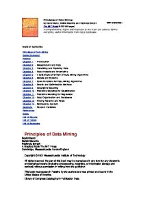
We are continually confronted with new phenomena. Sometimes it takes us years to build by hand a model that describes the observed phenomena and that allows us to predict new events. But more often there is an urgent need for such a model and the time to develop it is not given. These problems are known for example from medicine where we want to know how to treat people with a certain disease so that they can recover quickly. Years ago in 1993, we started out with data mining for a medical problem called in-vitro fertilization therapy (IVF therapy). We will take this problem as introductory example since it shows nicely how data mining can be applied and demonstrates the results that we can obtain from the data mining process [PeT97]. In-vitro fertilization therapy can help childless couples make their wish to have a baby come true. However, the success rate was very low in 1993. Although this therapy was already in use for more than ten years medical doctors had not been able to develop a clear model about the function and effect of the therapy. The main reason for that was seen in the complex interlocking of biological, clinical, and medical facts. Therefore, doctors started out to built up a database where each diagnostic parameter and clinical information of a patient was recorded. This data base contained parameters from ultra sonic images such as the number and the size of follicles recorded on certain days of the women menstruation’s cycle, clinical data, and hormone data. We used this data base and analyzed them with decision tree induction. As result we obtained a decision tree showing useful decision rules for the IVF-therapy, see Figure 1. This model contains rules such as for e.g.: IF hormone E2 at the third cycle day <=67 AND number of follicle <=16,5 AND hormone E2 at the 12. cycle day <= 2620 THEN Diagnosis_0. It described the diagnosis model in such a way that physicians could follow suit. The learnt decision tree had two functions for the physicians: 1. Exploratory Function The learnt rules helped the experts to better understand the effects of the therapy. This is possible since the knowledge is made explicit for the expert by the representation of the decision tree. He can understand the rules by tracing down each path of the decision tree. The trust in this knowledge got higher when he found among the whole set of rules a few rules that he had already built up in past. This knowledge gave him new impulses to think about the effects of the IVFP. Perner: Data Mining on Multimedia Data, LNCS 2558, pp. 1−11, 2002.  Springer-Verlag Berlin Heidelberg 2002

2

1 Introduction

therapy as well as to acquire new necessary information about the patient in order to improve the success rate of the therapy. 2. Prediction Function After some experiments we came up with a good model for a sub-diagnosis task of IVF-therapy. It is called diagnosis of over stimulation syndrome. Physicians could use the learnt model in order to predict the development of an over stimulation syndrome for new incoming patients. The attentive reader would have noted that we could not revolutionize the whole IVF-therapy. Our experiments at that time showed that the recent diagnostic measurements are not enough to characterize the whole IVF process. Nevertheless, results were enough to stimulate new discussion and gave new impulses for the therapy. --155 DS E2ZT3

<=67 74 DS ATZT12

>67 81 DS [0]

<=16.5 53 DS E2ZT12

<=2620 29 DS [0]

>16.5 21 DS LHZT3

>2620 24 DS E2ZT12

<=3600 5 DS [1]

<=2.69 15 DS [1]

>3600 19 DS E2ZT6

<=304.5 13 DS [0]

<=40 4 DS [1]

>40 2 DS [0]

>304.5 6 DS E2ZT3

<=50 4 DS [0]

Attributes

>2.69 6 DS E2ZT3

>50 2 DS [1]

Description

E2D ay_3, 6, 9, 12

Hormone Estradiol measured at Day 3, 6, 9, and 12 of the womans menstruation cycle

LHZ D ay 3

Luteinisierndes H ormone at the cycle day 3

Fig. 1. Data and results of IVF therapy

The application we have described before follows the empirical cycle of theory formation, see Figure 2. By collecting observations from our universe and analyzing these observations based on sound mathematical methods we can come up with a theory that allows us to predict new events about the universe. That is not only applicable to our introductory example it can be used for every application that meets the criteria of the empirical cycle.

1.2 Some More Real-World Applications

3

Prediction

Universe Theory

Analysis Observations

Fig. 2. Empirical Cycle of Theory Formation

1.1 What Is Data Mining? In our IVF example we discovered diagnosis knowledge from a set of data recorded from all patients based on Data Mining. By summarizing these data into a set of rules our method helped human to find the general meaning of the single data. Usually, humans built up such knowledge by experience over years. The task gets much harder as more complex the problem is. The IVF example is described by only 36 parameters. Sometimes there can be more than 100 parameters. This is not anymore to overlook by humans. The innovative idea of data mining is that it provides methods and systems that can automatically find these general meanings based on large and complex, digital recorded data. The data mining systems usually do not care about the number of parameters. They can work with 10 or even with several hundred parameters. However, our introductory example also showed that it is not always possible to come up with generalizations even when data are available. There must be generalization capability within the data. Otherwise, it can be already useful to find patterns in the data and use them for exploration purpose. This is a much weaker approach but useful for humans knowledge discovery process. For a formal definition of Data Mining we like to follow Gregory PiateskyShapiro’s definition: "Data Mining, which is also referred to as knowledge discovery in data bases, means a process of nontrivial extraction of implicit, previously unknown and potentially useful information (such as knowledge rules, constraints, regularities) from data in databases."

1.2 Some More Real-World Applications Say you have generated a record in a database listing all car insurance policy holders by age, sex, marital status and selected policy, for example, see Figure 3 and Figure 4. With Data Mining, you can use this database to generate knowledge

4

1 Introduction

telling you which market grouping buys which type of insurance policy. This knowledge allows you to adjust your product portfolio in order to supply gaps in demand or predict which product a new customer is most likely to opt for. Sex female female female male male male female male female female male female male female ...

Age 33 35 36 29 33 35 35 35 35 44 46 48 50 52 ...

Marital_Status Children single single single single single single single single single maried maried maried maried maried ... ...

Fig. 3. Exerpt of a customer data base

--18 DS MARITAL_ST

=single 13 DS CHILDREN

<=0 11 DS SEX

=female 5 DS ??? [ 1]

=married 5 DS [ 2]

>0 2 DS [ 2]

=male 6 DS ??? [ 1]

Fig. 4. Resulting decision tree for customer profiling

MAILPX 0 0 0 0 0 1 1 0 0 1 1 0 0 0

Purchase 1 1 1 1 1 1 1 1 1 1 1 1 1 1

...

1 1 1 1 1 2 2 2 2 2 2 2 2 2 ...

1.2 Some More Real-World Applications

5

Or a criminal investigation office generates a data pool of criminal offences containing information on the offender such as age, sex, behavior and relationship between victim and offender. With Data Mining, these databases can be used to establish offender profiles, which are useful in criminal investigations for narrowing down lists of suspects. Say a doctor has generated a database for a certain disease in which to store patients’ data along with clinical and laboratory values and details of the nature of the disease. With Data Mining techniques, he can use this data collection to acquire the knowledge necessary to describe the disease. This knowledge can then be used to make prognoses for new patients or predict likely complications. Figure 5 illustrates this process for the prediction of the day of the infection after liver transplantation.

Fig. 5. Illustration of the data and the data mining process for mining the knowledge for the identification of the time of infection after liver transplantation

6

1 Introduction

1.3 Data Mining Methods – An Overview 1.3.1 Basic Problem Types Data Mining methods can be distinguished into two main categories of data mining problems: 1. Prediction and 2. Knowledge Discovery (see Figure 6). While prediction is the strongest goal, knowledge discovery is the weaker approach and usually prior to prediction. The over-stimulation syndrome recognition described in Section 1 belongs to predictive data mining. In this example, we mined our data base for a set of rules that describes the diagnosis knowledge. The doctors use this knowledge for the prediction of the over-stimulation syndrome when a new patient comes in. Data Mining Method

Prediction

Classification

Regression

Knowledge Discovery

Deviation Detection

Clustering

Association Rules

Visualization

Fig. 6. Types of Data Mining Methods

For that kind of data mining, we need to know the classes or goals our system should predict. In most cases we might know a-priori these goals. However, there are other tasks were the goals are not known a-priori. In that case, we have to find out the classes based on methods such as clustering before we can go into predictive mining. Furthermore, the prediction methods can be distinguished into classification and regression while knowledge discovery can be distinguished into: deviation detection, clustering, mining associate rules, and visualization. To categorize the actual problem into one of these problem types is the first necessary step when dealing with Data Mining. Therefore, we will give a short introduction to the different methods. 1.3.2 Prediction 1.3.2.1 Classification Assume there is a set of observations from a particular domain. Among this set of data there is a subset of data labelled by class 1 and another subset of data labelled by class 2. Each data entry is described by some descriptive domain variables and

1.3 Data Mining Methods – An Overview

7

the class label. We now want to find a mapping function that allows to separate samples belonging to class 1 from those belonging to class 2. Furthermore, this function should allow to predict the class membership of new formerly unseen samples. Such kind of problems belong to the problem type "classification". There can be more than two classes but for simplicity we are only considering the two class problem. The mapping function can be learnt by decision tree or rule induction [WeK90], neural networks [Rze98][ShT02], statistical classification methods [CADKR02] or case-based reasoning [CrR02]. We will concentrate in this book on symbolical learning methods such as decision tree and rule induction and casebased reasoning. 1.3.2.2 Regression Whereas classification determines the set membership of the samples, the answer of regression [RPD98][AtR00] is numerical. Suppose we have a CCD sensor. We give light of a certain luminous intensity to this sensor. Then this light is transformed into a gray value by the sensor, according to a transformation function. When we change the luminous intensity, we also change the gray value. That means the variability of the output variable will be explained based on the variability of one or more input variables. 1.3.3 Knowlegde Discovery 1.3.3.1 Deviation Detection Real-world observation are random events. The determination of a characteristic values, such as the quality of an industrial part, the influence of a medical treatment to a patient group or the detection of visual attentive regions in images can be done based on statistical parameter tests. Methods for the estimation of unknown parameters, test of hypothesis and the estimation of confidence intervals in linear models can be found in Koch [Koc02]. 1.3.3.2 Cluster Analysis A number of objects that are represented by a n-dimensional attribute vector should be grouped into meaningful groups. Objects that get grouped into one group should be as similar as possible. Objects from different groups should be as dissimilar as possible. The basis for this operation is a concept of similarity that allows us to measure the closeness of two data entries and to express the degree of their closeness. In Chapter 3 Section 3.3.1-3.3.3 we will describe different similarity measures. Once groups have been found we can assign class labels to these groups and label each data entry in our data base according to its group membership with the corresponding class label. Then we have a data base which can serve as basis for classification.

8

1 Introduction

1.3.3.3 Visualization The famous remark "A picture is worth more than a thousand words." especially holds for the exploration of large data sets. Numbers are not easy to be overlooked by humans. The summarization of these data into a proper graphical representation may give humans a better insight into the data [EFP01]. For example, clusters are usually numerical represented. The dendrogram (see Figure 11) illustrates these groupings, and gives a human an understanding of the relations between the various groups and subgroups. A large set of rules is easier to understand when structured in a hierarchical fashion and graphically viewed such as in the form of a decision tree.

1.3.3.4 Association Rules To find out associations between different types of information which seem to have no semantic dependence can give useful insights in for e.g. customer behavior. Marketing manager have found that customer who buy oil will also by vegetables. Such information can help to arrange a supermarket so that customers feel more attract to shop there. To discover which HTML documents are retrieved in connection with other HTML documents can give insight in the user profile of the website visitors. We can identify lesioned structures in brain MR images. The existence of a lesioned area may suggest the existence of another leasioned structure having a distinct spatial relation to the other structure. To count the occurrences of such a pattern may give hints for the diagnosis. Methods on association rule mining can be found in Zhang et al. [ZhZ02] and Adamo [Ada01]. In [HGN02] are described the application of these methods to engineering data. 1.3.3.5 Segmentation Suppose we have mined a marketing data base for user profiles. In the next step, we want to set up a mailing action in order to advertise a certain product for which it is highly likely that it attracts this user group. Therefore, we have to select all addresses in our data base that meet the desired user profile. By using the learnt rule as query to the data base we can segment our data base into customer that do not meet the user profile and into those that meet the user profile. Or suppose we have mined a medical data base for patient profiles and want to call in these patients for a specific medical test. Then, we have to select the names and addresses of all patients from our data base that meet our patient profile. The separation of a database into only those data that meet a given profile is called segmentation.

1.4 Data Mining Viewed from the Data Side

9

1.4 Data Mining Viewed from the Data Side We have discussed data mining from the problem-type perspective. We can also view Data Mining from the data-type dimension. Although, mining text or images can be of the same problem type there have been developed over time special fields such as text mining [Vis01], time series analysis [SHS00], image mining [Per01], or web mining [KMSS02][BlG02][PeF02]. The specific problem for this type of data lies in the preparation of the data for the mining process and the representation of these data. Although the pixel of a 2D or 3D image are of numerical data type, it would not be wise to take the whole image matrix itself for the mining process. Usually, the original image might be distorted or corrupted by noise. By pre-processing the image and extracting higher-level information from the image matrix the influence of noise and distortions will be reduced as well as the number of information that have to be handled. Beyond this, the extraction of higher level information allows an understanding of the image content. The representation of an image can be done on different levels that are described in Chapter 2 Section 2.7.1. The categorization of text into similar groups or classification of text documents requires an understanding of the content of the documents. Therefore, the document has to go through different processing steps depending on the form of the available text. A printed document must be converted into a digital document that requires digitalization of the document, recognition of the printed area and the characters, grouping of the characters into words and sentences. A digital version must be parsed into words and all unnecessary formatting instructions must be removed. After all that we are still faced with the problem of the contextual word sense or the semantic similarity between different word. An application for text mining can be found in Visa et al. [VTVB02]. Types of Data

Time Series

Images

Sound Traffic Data Life Monitoring Medical Data

2D Images 3D Images

Time Series Analysis

Image Mining

Video

Text

Sever Logs WebDocuments

Handwrittings Documents

Video Mining

Text Mining

WebMining

Fig. 7. Overview of Data Mining Methods viewed from the Data Side

In time-series analysis the problem is to recognize events. That raises the question what is an event. Usually, changes from normal status will be detected by regres-

10

1 Introduction

sion. However, a time series can also be converted into a symbolic curve description and this representation can be the basis for the mining process [SchG02]. The basis for web mining are the server logs or the web documents. The necessary information must be extracted from both data types by parsing these documents. The final representation of multimedia data can be either of the type numerical or symbolical attributes but more complex representations such as e.g. strings, graphs, and relational structures are also possible.

1.5 Types of Data An overview about types of data is given in Figure 8. Attributes can be of numerical or categorical data type. Numerical variables are for example the temperature or the gray level of a pixel in an image. This variable can have distinct gray levels ranging from 0 to 255. Categorical data is one for which the measurement scale consists of a set of categories. For instance, the size of an object may be described as "small", "medium", and "big". There are different types of categorical variables. Categorical variables for which levels do not have a natural ordering are called nominal. Many categorical variables do have ordered levels. Such variables are called ordinal. For instance, the gray level may be expressed by categorical levels such as "black", "gray", and "white". It is clear that the levels "black" and "white" stay on the opposite ends of the gray level scale whereas the level "gray" lies in between of both levels. An interval variable is one that has numerical distances between any two levels of the scale. In the measurement hierarchy, interval variables are highest, ordinal variables are next, and nominal variables are lowest. Only an attribute-based description might not be appropriate for multimedia applications. The global structure of a given object or a scene and the semantic information of the parts of the objects or the scene and their relation might require an attributed graph representation. We define an attributed graph as follows: Definition 1: W ... set of attribute values e.g.: W = {"dark_grey", "left_behind", "directly_behind", ...} A ... set of all attributes e.g.: A = {shape, object area, spatial_relationship, ...} b: A → W partial mapping, called attribute assignments B ... set of all attribute assignments over A and W.

1.6 Conclusion

11

A graph G = (N, p, q) consists of N ... finite set of nodes p : N → B mapping of attributes to nodes q : E → B mapping of attributes to edges, where E = (NxN)\IN and IN is the Identity relation in N. The nodes are for example the objects and the edges are the spatial relation between the objects. Each object has attributes which are associated to the corresponding node within the graph.

Types of Data

numerical

categorical

string

graph

interval

ordinal

nominal

attributed graph

Fig. 8. Overview Types of Data

1.6 Conclusion In this chapter we have explained what data mining is and we gave an overview about the basic methods. The diversity of applications that we have described should give you an idea where it can be reasonable to apply data mining methods in order to get new insights into the application. It should inspire you to think about using data mining techniques even for your application. Despite the basic methods for data mining we have viewed the field from the data side. When it comes to multimedia data such as images, video or audio more complex data structures than attribute-value pair representations are often required such as e.g. sequences or graphs. They require special algorithm for mining which will describe in Section 3.3.9 for graph clustering.

2 Data Preparation

Before going into our data mining experiment, we need to prepare the data in such a way that they are suitable for the data mining process. The operations for data preparation can be categorized as follows (see Fig. 9):

• • • • • • •

Data cleaning Normalization Handling noisy, uncertain and untrustworthy information Missing value handling Transformation Data Coding Abstraction Operations for Data Preparation

Standardization

Noisy, Uncertain Untrustworthy Data Handling

Smooting

Missing Value Handling

Transformation Coding

Abstraction

Outlier Detection

Fig. 9. Data Preparation Operations

2.1 Data Cleaning Most data mining tools require the data in a format such as shown in table 1. It is a simple table sheet where the first line describes the attribute names and the class attribute and where the following lines contain the data entries describing the case number and the attribute values for each attribute of a case. It is important to note that the inputted data should follow the predefined names and types for the attributes. No subjective description of the person who collected the data should be inserted into the data base nor should other vocabulary be used than predefined in advance. Otherwise, we would have to remove these information in a data cleaning step. Since data cleaning is a time-consuming process and often double work it is better to set up the initial data base in such a way that it can immediately be P. Perner: Data Mining on Multimedia Data, LNCS 2558, pp. 13−22, 2002.  Springer-Verlag Berlin Heidelberg 2002

14

2 Data Preparation

used for data mining. Recent work on data ware houses [Mad01] take into consideration this aspect. Table 1. Common Data Table

Case C_1 C_2

F_1 V11 V21

F_2 V12 V22

... ... ...

F_k V1k V2k

C_i

Vi1

Vi2

...

vik

2.2 Handling Outlier In almost all real world data, some can be found, which differ so much from the others as to indicate some abnormal source of error not contemplated in the theoretical discussions. The introduction of which into the investigations can only serve to perplex and mislead the inquirer. Uni-variate outliers are to recognize by using boxplots [Car00][ZRC98]. Figure 10 shows the boxplots for the feature_1 of the iris data set [Fis]. Each box represents the range of the feature values for one of the three classes. The median for each data samples is indicated by the black center line, and the first and third quartiles are the edges of the red area. The difference of the first and third quartile is known as the interquartile range (IRQ). The black lines above and under the red boxes represent the area within 1.5 times the inter-quartile range. Points at a greater distance from the median than 1.5 times the IRQ are plotted individually. These points represent potential outliers. The problem gets much harder if multivariate outlier should be recognized. Such kind of outlier can be detected by cluster analysis (see Chapter 3 for cluster analysis). Based on a proper similarity measure the similarity of one sample to all the other samples is calculated and then visualized in a dendrogram by the single linkage method. Similar samples will form groups showing close relation to each other while outliers will result in single links showing a clear distance to the other groupings. A deeper insight to the handling of multi-variate outliers can be found in [BaT84][And84].

2.3 Handling Noisy Data Real measurements will usually be affected (corrupted) by noise. There are many reasons for noisy data. It can be caused by the measurement device, the environment or by the person who collected the data. The data shown in Figure 11 are data from the IVF therapy. It shows the hormone status of a woman from day three until day fourteen of the woman’s menstruation cycle. Taking the real measurements for learning the model will result in a prediction system with lower accu-

2.3 Handling Noisy Data

15

racy than that learnt from the smoothed data. By calculating the sliding mean value and using these data for learning we can improve the accuracy of the learnt model.

Fig. 10. Boxplot of Iris Data Feature_1

1 4 0 00 1 2 0 00 1 0 0 00

Z yk lu s 1

8000

Z yk lu s 2

6000

Z yk lu s 1 *

4000

Z yk lu s 2 *

2000 0 3

4

6

7

8

E 2[ t ] =

Fig. 11. Data Smoothing

9

10

t+n

∑

11

12

1 ⋅ E 2[ i ] 2 n i=t − n

13

14

16

2 Data Preparation

2.4 Missing Values Handling There are many reasons for missing values in real world data bases: 1. The value might not be measured (neglect) or simply not inputted in the data base. 2. There might be some objective reason that the value could not be measured. 3. This can be because a patient did not want us to measure this value or a person did not want to answer the question in a questionnaire. Now, we are faced with the problem: How to deal with missing values? The simplest strategy would be to eliminate the data set. This is insufficient for small data bases even if only one value in a data entry is missing. Therefore, it might be better to insert a global constant for missing values. This would at least guarantee to use the data set. However, this strategy does not reflect the real domain distribution of the attribute value. This can only be achieved by considering the statistical properties of the samples. For the one-dimensional case, we can calculate the class conditional distribution of the attribute values of an attribute. The mean value of the class the sample belongs to can be inserted for the missing value. For the ndimensional case, we can search for similar data tuple and insert the feature value of the most similar data tuple for the missing value. However, here we need to define a proper similarity measure in order to find close data entries. This problem its not trivial (see Chapter Case-Based Reasoning).

2.5 Coding A data mining tool or a data mining technique might require only numerical values regardless of whether the data type is numerical or symbolical. Then it is necessary to code the categorical data. The simplest form of coding would be to assign to each categorical value a distinct numerical value such that e.g. an attribute "color" gets for the attribute values "green"=1, "blue"=2, and "red"=3. More sophisticated coding techniques can be taken from the coding theory.

2.6 Recognition of Correlated or Redundant Attributes Selecting the right set of features for classification is one of the most important problems in designing a good classifier. Very often we do not know a-priori what the relevant features are for a particular classification task. One popular approach to address this issue is to collect as many features as we can prior to the learning and data-modeling phase. However, irrelevant or correlated features, if present, may degrade the performance of the classifier. In addition, large feature spaces

2.7 Abstraction

17

can sometimes result in overly complex classification models that may not be easy to interpret. In the emerging area of data mining applications, users of data mining tools are faced with the problem of data sets that are comprised of large numbers of features and instances. Such kinds of data sets are not easy to handle for mining. The mining process can be made easier to perform by focussing on a subset of relevant features while ignoring the other ones. This process is called feature subset selection (see Chapter 3.6). In the feature subset selection problem, a learning algorithm is faced with the problem of selecting some subset of features upon which to focus its attention.

2.7 Abstraction 2.7.1 Attribute Construction Between the attributes A1,A2,...,Ak,...Ai,...,An in the data table there might exist different relations depending from the domain. Instead of taking the basic attributes it might be wise to explore these relations between the attributes based on domain knowledge before the data mining experiment and construct new but more meaningful attributes Anew=Ai°Ak. The result of the mining process will have higher explanation capability than those using the basic attributes. Thereby the relation ° can be any logical or numerical function. The initial data table of our IVF domain contained the attribute size_i for each i of the n follicle. The construction of a new attribute mean_follicle_size brought more meaningful results. 2.7.2 Images Suppose, we have a medical doctor who for example will make the lung of a patient visible by taking an X-ray. The resulting image enables him to inspect the lung for irregular tissues. He will make the decision about malignant or benign nodule based on some morphological features of the nodule that appeared in the image. He has built up this knowledge over years in practice. A nodule will be malignant if for e.g. the following rule is satisfied: if the structure inside the nodule is irregular and areas of calcifications appear and there are sharp margins then the nodule is malignant. An automatic image interpretation based on such a rule would only be possible after the image has passed through various processing steps. The image must automatically be segmented into objects and background, objects must be labelled and described by features, these features must be grouped into symbolic representations until the final result can be obtained based on such a rule as described above in an interpretation step. In opposition to that, to mine an image data base containing only images and no image descriptions for such kind of knowledge would require to extract automatically the necessary information from the image. This is a contradiction. We do not know in advance our important

18

2 Data Preparation

features of a collection of images nor do we know the way they are represented in the image. Recently, we know low-level features such as blobs, regions, ribbons, lines, and edges and we know how these features can be extracted from images, see Figure 12. However, features such as an "irregular structure inside the nodule" are not so called low-level features. It is even not really clear the way this feature is represented in an image. Therefore, there does not exist an algorithm yet that can extract this feature. On the base of low-level features we can calculate some high-level features but it is not possible to obtain all such features in this way. Therefore, we should also allow to input experts descriptions into an image data base. Besides that, we can describe an image by statistical properties which might also be necessary information. On the base of this discussion we can identify different ways of representing the content of an image that belongs to different abstraction levels. The higher the chosen abstraction level is the more useful is the derived information with data mining. We can describe an image

• by statistical properties that is the lowest abstraction level, • by low-level features and their statistical properties such as regions, blobs, ribbons, edges and lines, which is the next higher abstraction level • by high-level or symbolic features that can be obtained from low-level features, and • at least by experts symbolic description which is the highest abstraction level. For the operations on images we like to refer the interested reader to special literature on image processing. For image preprocessing and segmentation see [PeB99]. The extraction of low-level features is described in [Zam96]. Texture description is described in [Rao90]. Image Statistics are described in [PeB99]. For an example on motion analysis see Imiya et al. [ImF99]. Examples for texture features and statistical features that can be used to describe the image content will be given in Chapter 4 based on two different applications. 2.7.3 Time Series Time series analysis is often referred to in the literature as event recognition [SrG99][FaF99]. For that purpose regression is used. However, the analysis of time series can also be concerned with interpretation such as scintigram analysis or noise analysis of technical objects. In medical processes doctors usually have to observe time series of several diagnostic parameters. Only the combination of these events in the different time series and their relation to each other can predict the occurrence of a disease or a dangerous status for patients. Such an analysis requires a temporal abstraction of the time series [Sha97][Sha99].

2.7 Abstraction

Feature Filter_1

Image

Segmentation & Object Labelling

Feature Filter_2 Feature Filter_3

Blobs

19

Description

Regions

Description

Ribbons

Calculationo f high-level Features

Description

... Feature Filter_n

Edges/Lines

Description

Symbolic Terms Spatial Relations

geometrical statistical properties texture, color

Description

low-level Features

Manual Acquisition Experts Description

Automatic Acquisition Pixel Statistical Description of Image

Numerical Features

Symbolic Description of Image

Image Mining Database Image _ 1 Image _ 2 ... Image _ N

Image Description Image Description ... Image Description

Fig. 12. Different Types of Information that can be extracted from Images

Time series can be described by parameters from the frequency or time domain, see Figure 13. We can use Fourier coefficients and the Ceptrum for the description of the time series. In the time domain we can describe a time series by curve segments of an n-th order interpolation function such as e.g. lines and parabola. These curve segments can be labeled by symbolic terms such as slope, peak, or valley then we can symbolically interpret the line segment. 2.7.4 Web Data There are different types of data: user entry data, server logs, web documents and webmeta data.

20

2 Data Preparation

Descripiton of Time Series

Time Domain

Frequency Domain

Fourier Analysis

Ceptrum Correlation Analysis

Interpolation

symbolical Description

Fig. 13. Description of Time Series

The user usually inputs user data himself when requested to register at a website or when he is answering a questionnaire on a website. These information are stored into a data base which can be taken later on for data mining. Web server logs are automatically generated by the server when a user is visiting an URL at a site. In a server log are registered the IP address of the visitor, the time when he is entering the website, the time duration he is visiting the requested URL and the URL he is visiting. From these information can be generated the path the user is going on this website [CMS99]. Web server logs are important information in order to discover the behavior of a user at the website. In the example given in Figure 15 a typical server log file is shown. Table 2 shows the code for the URL. In table 3 is shown the path the user is taking on this website. The user has been visiting the website 4 times. A user session is considered to be closed when the user is not taking a new action within 20 minutes. This is a rule of thumb that might not always be true. Since in our example the time duration between the first user access starting at 1: 54 and the second one at 2:24 is longer than 20 minutes we consider the first access and the second access as two sessions. However, it might be that the user was staying on this website for more than 20 minutes since he is not entering the website by the main page. The web documents contain information such as text, images, video or audio. They have a structure that allows to recognize for e.g. the title of the page, the author, keywords and the main body. The formatting instruction must be removed in order to access the information that we want to mine on these sides. An example of an HTML document is given in Figure 14. The relevant information on this page is marked with grey color. Everything else is HTML code which is enclosed into brackets <>. The title of a page can be identified by searching the page for the code to find the beginning of the title and for the code to find the end of the title. Images can be identified by searching the webpage for the file extension .gif, .jpg. Web meta data give us the topology of a website. This information is normally stored as a side-specific index table implemented as a directed graph.

2.7 Abstraction

welcome to the homepage of Petra Perner

Welcome to the homepage of Petra Perner

Industrial Conference Data Mining 24.7.-25.7.2001

In connection with MLDM2001 there will be held an industrial conference on Data Mining.

Please visit our website http://www.data-mining-forum.de for more information.

List of Accepted Papers for MLDM is now available. Information on MLDM2001 you can find on this site under the link MLDM2001

Fig. 14. Excerpt from a HTML Document hs2-210.handshake.de - - [01/Sep/1999:00:01:54 +0100] "GET /support/ HTTP/1.0" - "http://www.s1.de/index.html" "Mozilla/4.6 [en] (Win98; I)" Isis138.urz.uni-duesseldorf.de - - 01/Sep/1999:00:02:17 +0100] "GET /support/laserjet-support.html HTTP/1.0" - - "http://www.s4.de/support/" "Mozilla/4.0 (compatible; MSIE 5.0; Windows 98; QXW0330d)" hs2-210.handshake.de - - [01/Sep/1999:00:02:20 +0100] "GET /support/esc.html HTTP/1.0" - "http://www.s1.de/support/" "Mozilla/4.6 [en] (Win98; I)" pC19F2927.dip.t-dialin.net - - [01/Sep/1999:00:02:21 +0100] "GET /support/ HTTP/1.0" - "http://www.s1.de/" "MOZILLA/4.5[de]C-CCK-MCD QXW03207 (WinNT; I)" hs2-210.handshake.de - - [01/Sep/1999:00:02:22 +0100] "GET /service/notfound.html HTTP/1.0" - "http://www.s1.de/support/esc.html" "Mozilla/4.6 [en] (Win98; I)" hs2-210.handshake.de - - [01/Sep/1999:00:03:11 +0100] "GET /service/supportpack/ in dex_content.html HTTP/1.0" - - "http://www.s1.de/support/" "Mozilla/4.6 [en] (Win98; I)" hs2-210.handshake.de - - [01/Sep/1999:00:03:43 +0100] "GET /service/supportpack/kontakt.html HTTP/1.0" - - "http://www.s1.de/service/supportpack/index_content.html" "Mozilla/4.6 [en] (Win98; I)" cache-dm03.proxy.aol.com - - [01/Sep/1999:00:03:57 +0100] "GET /support/ HTTP/1.0" - "http://www.s1.de/" "Mozilla/4.0 (compatible; MSIE 5.0; AOL 4.0; Windows 98; DigExt)"

Fig. 15. Excerpt from a Server Logfile

21

22

2 Data Preparation

Table 2. URL Address and Code for the Address

URL Address www.s1.de/index.html www.s1.de/support/ www.s1.de/support/esc.html www.s1.de/support/service-not found.html www.s1.de/service/supportpack/index_ content.html www.s1.de/service/supportpack/kontak t.html

Code A B C D E F

Table 3. User, Time and Path the User has taken on the Web-Site

User Name USER_1 USER_1 USER_1 USER_1

Time 1:54 2:20 -2:22 3:11 3:43 - 3:44

Path A BÅC B EÅF

2.8 Conclusions Useful results can only be obtained by data mining when the data are carefully prepared. Unnecessary data, noisy data or even correlated data highly affect the result of the data mining experiment. Their influence should be avoided by applying proper data preparation techniques. The raw data of a multimedia source such as images, video, or logfile data cannot be used from scratch. Usually these data need to be transformed into a proper abstraction level. For example from an object in an image features should be calculated that describe the properties of the object. Each image will then have an entry in the data table containing the features of the objects extracted from the image. How the image should be represented is often domain-dependent and requires a careful analysis of the domain. We will show on examples in the chapter 4 how this can be done for different abstraction levels.

3 Methods for Data Mining

3.1 Decision Tree Induction 3.1.1 Basic Principle With decision tree induction we can automatically derive from a set of single observations a set of rules that generalizes these data (see Figure 16). The set of rules is represented as decision tree. Decision trees recursively partitions the solutions space based on the attribute splits into subspaces until the final solutions is reached. The resulting hierarchical representation is very natural to human problem solving process. During the construction of the decision tree are selected from the whole set of attributes only those attributes that are most relevant for the classification problem. Once the decision tree has been learnt and the developer is satisfied with the quality of the learnt model. This model can be used in order to predict the outcome for new samples. This learning methods is also called supervised learning since samples in the data collection have to be labelled by the class. Most decision tree induction algorithm allow to use numerical attributes as well as categorical attributes. Therefore, the resulting classifier can make the decision based on both types of attributes.

Class

SepalLeng SepalWi PetalLen PetalWi

Setosa

5,1

3,5

1,4

0,2

Setosa

4,9

3,0

1,4

0,2

Setosa

4,7

3,2

1,3

0,2

Setosa

4,6

3,1

1,5

0,2

Setosa

5,0

3,6

1,4

0,2

Versicolor

7,0

3,2

4,7

1,4

Versicolor

6,4

3,2

4,5

1,5

Versicolor

6,9

3,1

4,9

1,5

Versicolor

5,5

2,3

4,0

...

...

...

...

--150 DS PETALLEN

Decision Tree Induction

<=2.45 50 DS [Setosa ]

>2.45 100 DS PETALLEN

<=4.9 54 DS PETALWI

<=1.65 47 DS [Versicol]

1,3

>1.65 7 DS [Virginic]

...

Attribute-Value Pair Representation

Data Mining

Fig. 16. Basic Principle of Decision Tree Induction

P. Perner: Data Mining on Multimedia Data, LNCS 2558, pp. 23−89, 2002.  Springer-Verlag Berlin Heidelberg 2002

>4.9 46 DS [Virginic]

Result

24

3 Methods for Data Mining

3.1.2 Terminology of Decision Tree A decision tree is a directed a-cyclic graph consisting of edges and nodes, see Figure 17. The node with no edges enter is called the root node. The root node contains all class labels. Every node except the root node has exactly one entering edge. A node having no successor is called a leaf or terminal node. All other nodes are called internal nodes. The nodes of the tree contain the decision rules such as IF attribute A ≤ value THEN D. The decision rule is a function f that maps the attribute A to D. The sample set is splitted in each node into two subsets based on the constant value for the attribute. This constant is called cut-point. In case of a binary tree, the decision is either true or false. Geometrically, the test describes a partition orthogonal to one of the coordinates of the decision space. A terminal node should contain only samples of one class. If there are more than one class in the sample set we say there is class overlap. An internal node contains always more than one class in the assigned sample set. A path in the tree is a sequence of edges from (v1,v2), (v2,v3), ... , (vn-1,vn). We say the path is from v1 to vn and is of the length n. There is a unique path from the root to each node. The depth of a node v in a tree is the length of the path from the root to v. The height of node v in a tree is the length of a largest path from v to a leaf. The height of a tree is the height of its root. The level of a node v in a tree is the height of the tree minus the depth of v.

Root node_t i

terminal (class label)

C(t), F(t), D(t) k

j

Fig. 17. Representation of a Decision Tree

A binary tree is an ordered tree such that each successor of a node is distinguished either as a left son or a right son; no node has more than one left son nor more than one right son. Otherwise it is a multivariate tree. Let us now consider the decision tree learnt from Fisher´s Iris data set [Fisher]. This data set has three classes (1-Setosa, 2-Vericolor, 3-Virginica) with 50 observations for each class and four predictor variables (petal length, petal width, sepal length and sepal width). The learnt tree is shown in Figure 18. It is a binary tree. The average depth of the tree is 1+3+2=6/3=2. The root node contains the attribute

3.1 Decision Tree Induction

25

petal_length. Along a path the rules are combined by the AND operator. Following the two paths from the root node we obtain for e.g. two rules such as: Rule1: IF petal_lenght<=2.45 THEN Setosa Rule 2: IF petal_lenght<2.45 AND petal_lenght<4.9 THEN Virginica. In the later rule we can see that the attribute petal_length will be used two times during the problem solving process. Each time it is used a different cut-point on this attribute. This representation results from the binary tree building process since only axis-parallel decision surfaces (see Figure 21) based on single cutpoints are created. However, it only means that the values for an attribute should fall into the interval [2.45,4.9] for the desired decision rule. --150 DS PETALLEN

<=2.45 50 DS [Setosa ]

>2.45 100 DS PETALLEN

<=4.9 54 DS PETALWI

<=1.65 47 DS [Versicol]

>4.9 46 DS [Virginic]

>1.65 7 DS [Virginic]

Fig. 18. Decision Tree learnt from Iris Data Set

3.1.3 Subtasks and Design Criteria for Decision Tree Induction The overall procedure of the decision tree building process is summarized in Figure 19. Decision trees recursively split the decision space into subspaces based on the decision rules in the nodes until the final stopping criteria is reached or the remaining sample set does not suggest further splitting. For this recursive splitting the tree building process must always pick among all attributes that attribute which shows the best result on the attribute selection criteria for the remaining sample set. Whereas for categorical attributes the partition of the attributes values is given a-priori. The partition (also called attribute discretization) of the attribute values for numerical attributes must be determined.

26

3 Methods for Data Mining

do while tree termination criterion faild do for all features feature numerical? yes

no

splitting-procedure feature selection procedure split examples built tree

Fig. 19. Overall Tree Induction Procedure

It can be done before or during the tree building process [DLS95]. We will consider the case where the attribute discretization will be done during the tree building process. The discretization must be carried out before the attribute selection process since the selected partition on the attribute values of a numerical attribute highly influences the prediction power of that attribute. After the attribute selection criteria was calculated for all attributes based on the remaining sample set, the resulting values are evaluated and the attribute with the best value for the attribute selection criteria is selected for further splitting of the sample set. Then, the tree is extended by a two or more further nodes. To each node is assigned the subset created by splitting on the attribute values and the tree building process repeats. Attribute splits can be done:

• • •

univariate on numerically or ordinal ordered attributes X such as X <= a, multivariate on categorical or discretized numerical attributes such as X∈A, or linear combination split on numerically attributes ∑ a i X i ≤ c . i

The influence of the kind of attribute splits on the resulting decision surface for two attributes is shown in Figure 21. The axis-parallel decision surface results in a rule such as IF F3 ≥4.9 THEN CLASS Virginica while the linear decision surface results in a rule such as IF -3.272+0.3254*F3+F4 ≥ 0 THEN CLASS Virginica.

3.1 Decision Tree Induction

27

The later decision surface better discriminates between the two classes than the axis-parallel one, see Figure 21. However, by looking at the rules we can see that the explanation capability of the tree will decrease in case of the linear decision surface.

3,0 Attribute F4

2,5 2,0

Class Setosa Class Verisicolor Class Virginica

1,5 1,0 0,5 0,0 0,0

2,0

4,0

6,0

8,0

Attribute F3 Fig. 20. Axis-Parallel and linear Attribute Splits Graphically Viewed in Decision Space 3,0

1. Schritt

---

Klasse 3

150 DS F3

Attribut F4

2,5

2. Schritt

2,0

Klasse 1

Klasse

1,5

3

<=2.45

>2.45

50 DS [1]

100 DS F4

2

1,0

1

Klasse 2

,5 0,0 0

1

2

3

4

5

6

<=1.8

>1.8

50 DS [2]

50 DS [3]

7

Attribut F3

Fig. 21. Demonstration of Recursively Splitting of Decision Space based on two Attributes of the IRIS Data Set

The induced decision tree tends to overfit to the data. This is typically caused due to noise in the attribute values and class information present in the training set. The tree building process will produce subtrees that fit to this noise. This causes an increased error rate when classifying unseen cases. Pruning the tree which means replacing subtrees with leaves will help to avoid this problem.

28

3 Methods for Data Mining

Now, we can summarize the main subtasks of decision tree induction as follow:

• • •

attribute selection (Information Gain [Qui86], X -Statistic [Ker92], GiniIndex [BFO84], Gain Ratio [Qui88], Distance measure-based selection criteria [Man91], attribute discretization (Cut-Point [Qui86], Chi-Merge [Kerb92], MLDP [FaI93] , LVQ-based discretization, Histogram-based discretization, and Hybrid Methods [PeT98], and pruning (Cost-Complexity [BFO84], Reduced Error Reduction Pruning [Qui86], Confidence Interval Method [Qui87], Minimal Error Pruning [NiB81]). 2

Beyond that, decision tree induction algorithm can be distinguished in the way they access the data and in non-incremental and incremental algorithms. Some algorithms access the whole data set in the main memory of the computer. This is insufficient if the data set is very large. Large data sets of millions of data do not fit in the main memory of the computer. They must be assessed from disk or other storage device so that all these data can be mined. Accessing the data from external storage devices will cause long execution time. However, the user likes to get results fast and even for exploration purposes he likes to carry out quickly various experiments and compare them to each other. Therefore, special algorithm have been developed that can work efficiently although using external storage devices. Incremental algorithm can update the tree according to the new data while nonincremental algorithm go trough the whole tree building process again based on the combined old data set and the new data. Some standard algorithm are: CART, ID3, C4.5, C5.0, Fuzzy C4.5, OC1, QUEST, CAL 5. 3.1.4 Attribute Selection Criteria Formally, we can describe the attribute selection problem as follow: Let Y be the full set of features, with cardinality k, and let ni be the number of samples in the remaining sample set i . Let the feature selection criterion function for the attribute be represented by S(A,ni). Without any loss of generality, let us consider a higher value of S to indicate a good attribute A. Formally, the problem of attribute selection is to find an attribute A based on our sample subset ni that maximizes our criteria S so that

S ( A, ni ) = max S ( Z , ni )

(1)

Z ⊆Y , Z =1

Numerous attribute selection criteria are known. We will start with the most used criteria called information gain criteria.

3.1 Decision Tree Induction

29

3.1.4.1 Information Gain Criteria and Gain Ratio Following the theory of the Shannon channel [Phi87], we consider the data set as the source and measure the impurity of the received data when transmitted via the channel. The transmission over the channel results in the partition of the data set into subsets based on splits on the attribute values J of the attribute A. The aim should be to transmit the signal with the least loss on information. This can be described by the following criterion:

IF

I ( A) = I (C ) − I (C / J ) = Max THEN

Select

Attribute − A

where I(A) is the entropy of the source, I(C) is the entropy of the receiver or the expected entropy to generate the message C1, C2, ..., Cm and I(C/J) is the losing entropy when branching on the attribute values J of attribute A. For the calculation of this criterion we consider first the contingency table in table 4 with m the number of classes, n the number of attribute values J, n the number of examples, Li number of examples with the attribute value Ji, Rj the number of examples belonging to class Cj, and xij the number of examples belonging to class Cj and having attribute value Ai. Now, we can define the entropy of the class C by:

I (C ) = −

m Rj Rj • ld N j =1 N

∑

(2)

The entropy of the class given the feature values, is: n m Li m xij xij 1 n I (C / J ) = ∑ ⋅ ∑− ld = ∑Li logLi − ∑∑ xij logxij Li Li N i =1 i =1 N j =1 i =1 j =1 n

(3)

The best feature is the one that achieves the lowest value of (2) or, equivalently, the highest value of the "mutual information" I(C) - I(C/J). The main drawback of this measure is its sensitivity to the number of attribute values. In the extreme case, a feature that takes N distinct values for the N examples achieves complete discrimination between different classes, giving I(C/J)=0, even though the features may consist of random noise and be useless for predicting the classes of future examples. Therefore, Quinlan [Qui88] introducted a normalization by the entropy of the attribute itself:

30

3 Methods for Data Mining

n G(A)=I(A)/I(J) with I ( J ) = − ∑ Li ld Li i =1

N

(4)

N

Other normalization have been proposed by Coppersmith et. al [CHH99] and Lopez de Montaras [LoM91]. Comparative studies have been done by White and Lui [WhL94].

Table 4. Contingency Table for an Attribute

Class Attribute values J1 J2 . . . Ji . . . Jn SUM

C1 x11 x21 . . . xi1 . . . xn1 R1

C2 x12 x22 . . . xi2 . . . xn2 R2

... ... ... ... ... ... ... ... ... ... ... ...

Cj x1j x2j . . . xij . . . xnj Rj

... ... ... ... ... ... ... ... ... ... ... ...

Cm SUM x1m L1 x2m L2 . . . . . . xim Li . . . . . . xnm Ln Rm N

3.1.4.2 Gini Function This measure takes into account the impurity of the class distribution. The Gini function is defined as: m

G = 1 − ∑ pi2 i =1

The selection criteria is defined as:

IF Gini( A) = G(C) − G(C / A) = Max! THENSelect Attribute_ A

(5)

3.1 Decision Tree Induction

31

The Gini function for the class is:

 Rj G (C ) = 1 − ∑  j =1  N m

   

2

(6)

The Gini function of the class given the feature values is defined as: n

G (C / J ) = ∑ i =1

Li G( J i ) N

(7)

with

 x ij G ( J i ) = 1 − ∑  j =1  Li m

   

2

(8)

3.1.5 Discretization of Attribute Values A numerical attribute may take any value on a continuous scale between its minimal value x1 and its maximal value x2. Branching on all these distinct attribute values does not lead to any generalization and would make the tree very sensitive to noise. Rather we should find meaningful partitions on the numerical values into intervals. The intervals should abstract the data in such a way that they cover the range of attribute values belonging to one class and that they separate them from those belonging to other classes. Then, we can treat the attribute as a discrete variable with k+1 intervals. This process is called discretization of attributes. The points that split our attribute values into intervals are called cut-points. The cut-points k lies always on the border between the distribution of two classes. Discretization can be done before the decision tree building process or during decision tree learning [DLS95]. Here we want to consider discretization during the tree building process. We call them dynamic and local discretization methods. They are dynamic since they work during the tree building process on the created subsample sets and they are local since they work on the recursively created subspaces. If we use the class label of each example we consider the method as supervised discretization methods. If we do not use the class label of the samples we call them unsupervised discretization methods. We can partition the attribute values into two (k=1) or more intervals (k>1). Therefore, we distinguish between binary and multi-interval discretization methods, see Figure 23 . In Figure 22, we see the conditional histogram of the values of the attribute petal_length of the IRIS data set. In the binary case (k=1), the attribute values

32

3 Methods for Data Mining

would be splitted at the cut-point 2.35 into an interval from 0 to 2.35 and a second interval from 2.36 to 7. If we do multi-interval discretization, we will find another cut-point at 4.8. That groups the values into 3 intervals (k=2): intervall_1 from 0 to 2.35, interval_2 from 2.36 to 4.8, and interval_3 from 4.9 to 7. We will also consider attribute discretization on categorical attributes. Many attribute values of a categorical attribute will lead to a partition of the sample set into many small subsample sets. This again will result into a quick stop of the tree building process. To avoid this problem, it might be wise to combine attribute values into a more abstract attribute value. We will call this process attribute aggregation. It is also possible to allow the user to combine attribute interactively during the tree building process. We call this process manual abstraction of attribute values, see Figure 23. 16

14

12

Mean

10

8

6

Peaks

4

Klasse 1 Setosa

2

Klasse 2 Versicolor Klasse 3 Virginica

0 1,0

1,3

1,6

1,9

2,2

2,5

2,8

3,1

3,4

3,7

4,0

4,3

4,6

4,9

5,2

5,5

5,8

6,1

6,4

6,7

4,8

2,35

Cut-Points

Petal length

Fig. 22. Histogram of Attribute Petal Length and Cut-Points

Attribute Discretization

Numerical Attributes

Binary (Cut-Point Determination)

Multi-Interval Discretization

Categorical Attributes

Abstraction Manual based on Domain Knowledge

Automatic Aggregation

Fig. 23. Overview about Attribute Discretization

3.1.5.1 Binary Discretization 3.1.5.1.1 Binary Discretization Based on Entropy Decision tree induction algorithm like ID3 and C4.5 use an entropy criteria for the separation of attribute values into two intervals. On the attribute range between xmin

3.1 Decision Tree Induction

33

and xmax is tested each possible cutpoint T and the one that fullfils the following condition is chosen as cutpoint TA:

IF

I ( A, TA ; S ) = Min! THEN

Select TA

for T

with S the subsample set, A the attribute, and T the cutpoint that separates the samples into subset S1 and S2. I(A, TA; S) is the entropy for the separation of the sample set into the subset S1 and S2 :

I ( A; T ; S ) =

S S1 I (S1 ) + 2 I ( S 2 ) S S

(9)

m

I ( S ) = −∑ p (C i , S ) ld j =1

(10)

p (C i , S )

The calculation of the cut-point is usually a time consuming process since each possible cut-point is tested against the selection criteria. Therefore, algorithms have been proposed that speed up the calculation of the right cut-point [Sei93]. 3.1.5.1.2 Discretization Based on Inter- and Intra Class Variance To find the threshold we can also do unsupervised discretization. Therefore, we consider the problem as a clustering problem in a one-dimensional space. The ra2 tio between the inter-class variance sB of the two subsets S1 and S2 and the intra2 class variance sw in S1 and S2 is used as criteria for finding the threshold:

s B2 = P0 (mo − m) 2 + P1 (m1 − m) 2 and

sW2 = P0 s 02 + P1 s12

(11)

h( x i ) N

(12)

The variances of the two groups are defined as: T

s 02 = ∑ ( xi − m0 ) 2 i = x1

h( xi ) and N

x2

s12 = ∑ ( xi − m1 ) 2 i =T

with N the number of all samples and h(xi) the frequency of attribute value xi. T is the threshold that will be tentatively moved over all attribute values. The values m0 and m1 are the mean values of the two groups that give us:

m = m0 P0 + m1 P1 where P0 and P1 are the probability for the values of the subset 1 and 2:

(13)

34

3 Methods for Data Mining

T

h( xi ) and i = x1 N

P0 = ∑

x2

P1 = ∑ i =T

h( x i ) N

(14)

The selection criteria is:

IF

s B2 = MAX ! THEN Select TA for T s w2

3.1.5.2 Multi-interval Discretization Binary interval discretization will result in binary decision trees. This might not always be the best way to model the problem. The resulting decision tree can be very bushy and the explanation capability might not be good. The error rate might increase since the approximation of the decision space based on the binary decisions might not be advantageous and, therefore, leads to a higher approximation error. Depending on the data it might be better to create decision trees having more than two intervals for numerical attributes. For multi-interval discretization we have to solve two problems: 1. Find multi intervals and 2. 2. Decide about the sufficient number of intervals. The determination of the number of the intervals can be done static or dynamic. In the later case the number of intervals will be automatically calculated during the learning process whereas in the static case the number of intervals will be given a-prior by the user prior to the learning process. Then, the discretization process will calculate as much intervals as it reaches the predefined number regardless if the class distribution in the intervals is sufficient or not. This results in trees having always the same number of attribute partitions in each node. All algorithm described above can be taken for this discretization process. The difference between binary interval discretization is that this process does not stop after the first cut-point has been determined the process repeat until the given number of intervals is reached [PeT98] During dynamic discretization process are automatically calculated the sufficient number of intervals. The resulting decision tree will have different attribute partitions in each node depending on the class distribution of the attribute. For this process, we need a criterion that allows us to determine the optimal number of intervals.

3.1 Decision Tree Induction

35

3.1.5.2.1 Basic (Search Strategies) Algorithm Generally, we have to test any possible combinations of cut-points k in order to find the best cut-points. This would be computational expensive. Since we assume that cut-points are always on the border of two distributions of x given class c, we have a heuristic for our search strategy. Discretization can be done bottom-up or top-down. In the bottom-up case, we will start with a finite number of intervals. In the worst case, these intervals are equivalent the original attribute values. They can also be selected by the user or estimated based on the maximum of the second order probability distribution that will give us a hint where the class borders are located. Starting from that the algorithm merges intervals that do met the merging criteria until a stopping criteria is reached. In the top-down case, the algorithm first selects two intervals and recursively refines these intervals until the stopping criteria is reached. 3.1.5.2.2 Determination of the Number of Intervals In the simplest case the user will specify how many intervals should be calculated for a numerical attribute. This procedure might become worse when there is no evidence for the required number of intervals in the remaining data set. This will result in bushy decision trees or will stop the tree building process sooner as possible. Much better would be to calculate the number of intervals from the data. Fayyad and Irani [FaI93] developed a stopping criteria based on the minimum description length principle. Based on this criteria the number of intervals is calculated for the remaining data set during decision tree induction. This discretization procedure is called MLD-based discretization. Another criteria can use a cluster utility measure to determine the best suitable number of intervals [Per00]. 3.1.5.2.3 Cluster Utility Criteria Based on the inter-class variance and the intra-class variance we can create a cluster utility measure that allows us to determine the optimal number of intervals. We assume that inter-class variance and intra-class variance are the inter-interval variance and intra-interval variance. 2

Let s w be the intra-class variance and can define our utility criteria as follow: n

U=

∑s k =1

2 wk

s B2 be the inter-class variance. Then we

− sbk2

n

The number of intervals n is chosen for minimal U.

(15)

36

3 Methods for Data Mining

3.1.5.2.4 MLD Based Criteria The MLD-based criteria was introduced by Fayyad and Irani [FaI92] Discretization is done based on the gain ratio. The gain ratio I(A, T;S) (see Section) is tested after each new interval against the MLD-criteria:

I ( A, T ; S ) >

log 2 ( N − 1) ∇( A, T ; S ) + N N

(16)

where N is the number of instances in the set S and

(

)

∇( A, T ; S ) = log 2 3 k − 2 − [k ⋅ I ( S ) − k1 ⋅ I ( S1 ) − k 2 I ( S 2 )]

(17)

One of the main problems with this discretization criteria is that it is relatively expensive. It must be evaluated N-1 times for each attribute (with N the number of attribute values). Typically, N is very large. Therefore, it would be good to have an algorithm which uses some assumption in order to reduce the computation time. 3.1.5.2.5 LVQ-Based Discretization Vector quantization is also related to the notion of discretization [PeT98]. for our experiment. LVQ [Koh95] is a supervised learning algorithm. This method attempts to define class regions in the input data space. Firstly, a number of codebook vectors Wi labeled by a class are placed into the input space. Usually several codebook vectors are assigned to each class. The learning algorithm is realized as follow: After an initialization of the neural net, each learning sample is presented one or several times to the net. The input vector X will be compared to all codebook vectors W in order to find the closest codebook vector Wc. The learning algorithm will try to optimize the similarity between the codebook vectors and the learning samples by shifting the codebook vectors in the direction of the input vector if the sample represents the same class as the closest codebook vector. In case of the codebook vector and the input vector having different classes the codebook vector gets shifted away from the input vector, so that the similarity between these two decrease. All other code book vectors remain unchanged. The following equations represent this idea:

[

for equal classes: Wc (t + 1) = Wc (t ) + α (t ) ⋅ X (t ) − Wc (t )

[

]

for different classes: Wc (t + 1) = Wc (t ) − α (t ) ⋅ X (t ) − Wc (t ) For all other: Wj (t + 1) = Wj (t )

(18)

]

(19) (20)

3.1 Decision Tree Induction

37

This behavior of the algorithms we can employ for discretization. A potential cut point might be in the middle of the learned codebook vectors of two different classes. Figure 24 shows this method based on one attribute of the IRIS domain. Since this algorithm tries to optimize the misclassification probability we expect to get good results. However, the proper initialization of the codebook vectors and the choice of learning rate α (t ) is a crucial problem. 16

14

12

Mean

10

8

6

4 Klasse 1 Setosa

2

Klasse 2 Versicolor Klasse 3 Virginica

0 1,0

1,3

1,6

1,9

2,2

2,5

2,8

3,1

3,4

3,7

4,0

4,3

4,6

4,9

5,2

5,5

5,8

6,1

6,4

6,7

1,0

1,3

1,6

1,9

2,2

2,5

2,8

3,1

3,4

3,7

4,0

4,3

4,6

4,9

5,2

5,5

5,8

6,1

6,4

6,7

Codebook vectors

Petal length

Fig. 24. Class Distribution of an Attribute and Codebook Vectors

3.1.5.2.6 Histogram Based Discretization A histogram-based method has been suggested first by Wu et al. [WLS75]. They used this method in an interactive way during top-down decision tree building. By observing the histogram, the user selects the threshold which partitions the sample set in groups containing only samples of one class. In Perner et al. [PeT98] is described an automatic histogram-based method for feature discretization. The distribution p(a|a³Ck)P(Ck) of one attribute a according to classes Ck is calculated. The curve of the distribution is approximated by a first order polynom and the minimum square error method is used for calculating the coefficients:

E=

∑ (a x i =1

1

i

+ a0 − yi ) 2

n

a1 =

∑x i =1 n

i

∑i i =1

(21)

⋅i (22) 2

38

3 Methods for Data Mining

The cut points are selected by finding two maxima of different classes situated next to each other. We used this method in two ways: First, we used the histogram-based discretization method as described before. Second, we used a combined discretization method based on the distribution p(a|a³Sk)P(Sk) and the entropy-based minimization criteria. We followed the corollary derived by Fayyad and Irani [FaI93], which says that the entropy-based discretization criteria for finding a binary partition for a continuous attribute will always partition the data on a boundary point in the sequence of the examples ordered by the value of that attribute. A boundary point partitions the examples in two sets, having different classes. Taking into account this fact, we determine potential boundary points by finding the peaks of the distribution. If we found two peaks belonging to different classes, we used the entropy-based minimization criteria in order to find the exact cut point between these two classes by evaluation each boundary point K with Pi ≤ K ≤ Pi+1 between this two peaks. 16

14

12

Mean

10

8

6

Peaks

4

Klasse 1 Setosa

2

Klasse 2 Versicolor Klasse 3 Virginica

0 1,0

1,3

1,6

1,9

2,2

2,5

2,8

3,1

3,4

3,7

4,0

4,3

4,6

4,9

5,2

5,5

5,8

6,1

4,8

2,35

6,4

6,7 Cut-Points

Petal length

Fig. 25. Examples sorted by attribute values for attribute A and labelled peaks

This method is not as time consuming like the other ones. We wanted to see if this method can be an alternative to the methods described before and if we can find a hybrid version which combines the advantages of the low computation time of the histogram-based method with the entropy minimization heuristic in the context of discretization. 3.1.5.2.7 Chi-Merge Discretization The ChiMerge algorithm introduced by Kerber [Ker92] consists of an initialization step and a bottom-up merging process, where intervals are continuously merged until a termination condition is met. Kerber used the ChiMerge method static. In our study we apply ChiMerge dynamically to discretization. The poten2 tial cut-points are investigated by testing two adjacent intervals by the c independence test. The statistical test values is:

3.1 Decision Tree Induction

m

k

χ = ∑∑ 2

i =1 j =1

( Aij − Eij )2

39

(23)

Eij

where m=2 (the intervals being compared), k - number of classes, Aij - number of examples in i-th interval and j-th class, Ri - number of examples in i-th interval m

k

Ri = ∑ Aij ; Cj - number of examples in j-th class C j = ∑ Aij ; N – the total i =1

j =1

number of examples

k

Ri ⋅ C j

j =1

N

N = ∑ C j ; Eij -expected frequency Eij =

.

Firstly, all boundary points will used for cut-points. In the second step for each pair of adjacent intervals one compute the χ²-value. The two adjacent intervals with the low-est χ²-value will merge together. This step is repeated continuously until all χ²-value exceeding a given threshold. The value for the threshold is determined by selecting a desired significance level and then using a table or for2 mula to obtain the c . 3.1.5.2.8 The Influence of Discretization Methods on the Resulting Decision Tree Figure 26-29 show decision trees learnt based on different discretization methods. It shows that the kind of discretization method influences the attribute selection. The attribute in the root node is the same for the decision tree based on Chi-Merge discretization (see Figure 26) and LVQ-based discretization (see Figure 28). The calculated intervals are rawly the same. Since the tree generation based on histogram discretization requires always two cut-points and since in the remaining sample set is no evidence for two cut-points the learning process stops after the first level. The two trees generated based on Chi-Merge discretization and on LVQ-based discretization have also the same attribute in the root. The intervals are also slightly differently selected by the two methods. The tree in Figure 28 is the most bushy tree. However, the error rate (see Table 3.1.2) of this tree calculated based on leave-one out (see Chapter) is not better than the error rate of the tree shown in Figure 27. Since the decision is based on more attributes (see Figure 28) the experts might like this tree much more than the tree shown in Figure 29.

40

3 Methods for Data Mining

--150 DS PETALWI

<=0.8 50 DS [Setosa ]

>0.8 & <=1.75 54 DS ??? [Versicol]

>1.75 46 DS ??? [Virginic]

Fig. 26. Decision Tree based on Chi-Merge Discretization (k=3)

--150 DS PETALLEN

<=2.45 50 DS [Setosa ]

>2.45 & <=4.95 54 DS ??? [Versicol]

>4.95 46 DS ??? [Virginic]

Fig. 27. Decision Tree based on Histogram based Discretization (k=3) --150 DS PETALWI

<=0.8375 50 DS [Setosa ]

>0.8375 & <=1.6375 52 DS PETALLEN

<=5.04864 48 DS SEPALWI

<=2.275 4 DS PETALWI

<=1.4375 2 DS [Versicol]

>2.275 44 DS [Versicol]

>1.6375 48 DS PETALLEN

>5.04864 4 DS SEPALLENG

<=6.1875 2 DS ??? [Versicol]

>6.1875 2 DS [Virginic]

>1.4375 2 DS ??? [Versicol]

Fig. 28. Decision Tree based on LVQ based Discretization

<=5.025 10 DS SEPALWI

<=2.9625 6 DS [Virginic]

>5.025 38 DS [Virginic]

>2.9625 4 DS SEPALLENG

<=6.0875 2 DS ??? [Versicol]

>6.0875 2 DS ??? [Versicol]

3.1 Decision Tree Induction

41

--150 DS PETALLEN

<=2.45 50 DS [Setosa ]

>2.45 & <=4.9 54 DS PETALWI

<=1.65 47 DS [Versicol]

>4.9 46 DS ??? [Virginic]

>1.65 7 DS ??? [Virginic]

Fig. 29. Decision Tree based on MLD-Principle Discretization Table 5. Error Rate for Decision Trees based on different Discretization Methods

Descritization Method Chi-Merge Histogram based Discr. LVQ based Discr. MLD-based Discr.

Error Rate Unpruned Tree

Pruned Tree

6 4 4

6 5.33 4

3.1.5.3 Discretization of Categorical or Symbolical Attributes

3.1.5.3.1 Manual Abstraction of Attribute Values In opposition to numerical attributes, symbolical attributes may have a large number of attribute values. Branching on such an attribute causes a partition into small sub sample sets that will often lead to a quick stop of the tree building process or even to trees with low explanation capabilities. One way to avoid this problem is the construction of meaningful abstractions on the attribute level at hand based on a careful analysis of the attribute list [PBY96]. This has to be done in the preparation phase. The abstraction can only be done on the semantic level. Advantageous is that the resulting interval can be named with a symbol that human can understand.

3.1.5.3.2 Automatic Aggregation However, it is also possible to do automatically abstraction on symbolical attribute values during the tree building process based on the class-attribute interdepend-

42

3 Methods for Data Mining

ence. Then the discretization process is done bottom-up starting from the initial attribute intervals. The process stops until the criteria is reached. 3.1.6 Pruning If the tree is allowed to grow up to its maximum size it is likely that it becomes overfitted to the training data. Noise in the attribute values and class information will amplify this problem. The tree building process will produce subtrees that fit to noise. This unwarranted complexity causes an increased error rate when classifying unseen cases. This problem can be avoided by pruning the tree. Pruning means replacing subtrees by leaves based on some statistical criterion. This idea is illustrated in Figure 30 and Figure 31 on the IRIS data set. The unpruned tree is a large and bushy tree with an estimated error rate of 6.67%. Up to the second level of the tree gets replaced subtrees by leaves. The resulting pruned tree is smaller and the error rate becomes 4.67% calculated with cross validation. Pruning methods can be categorized either in pre- or post-pruning methods. In pre-pruning, the tree growing process is stopped according to a stopping criteria before the tree reaches its maximal size. In contrast to that, in post-pruning, the tree is first developed to its maximum size and afterwards, pruned back according to a pruning procedure. --150 DS PETALLEN

<=2.45 50 DS [Setosa ]

>2.45 100 DS PETALLEN

<=4.9 54 DS PETALWI

<=1.65 47 DS [Versicol]

>4.9 46 DS PETALWI

>1.65 7 DS SEPALLENG

<=5.95 3 DS ??? [Virginic]

<=1.75 6 DS PETALLEN

>5.95 4 DS [Virginic]

<=5.1 4 DS PETALWI

<=1.55 2 DS [Virginic]

Fig. 30. Unpruned Decision Tree for the IRIS Data Set

>1.75 40 DS [Virginic]

>5.1 2 DS [Virginic]

>1.55 2 DS [Versicol]

3.1 Decision Tree Induction

43

--150 DS PETALLEN

<=2.45 50 DS [Setosa ]

>2.45 100 DS PETALLEN

<=4.9 54 DS PETALWI

<=1.65 47 DS [Versicol]

>4.9 46 DS [Virginic]

>1.65 7 DS [Virginic]

Fig. 31. Pruned Tree for the IRIS Data Set based on Minimal Error Pruning

3.1.7 Overview Post-Pruning methods can be mainly categorized into methods that uses an independent pruning set and those that uses no separate pruning set, see Figure 32. The later one can be further distinguished into methods that uses traditional statistical measures, re-sampling methods like crossvalidation and bootstrapping, and codelenght motivated methods. Here we only want to consider cost-complexity pruning and confidence interval pruning that belongs to the methods with separate pruning set. An overview about all methods can be found in Kuusisto [Kuu98]. Pruning Methods

Uses Independent Pruning Set

No Separate Pruning Set

Resampling Methods

Codelength Motivated Pruning Methods

Statistical Methods

Fig. 32. General Overview about Pruning Methods

3.1.8 Cost-Complexity Pruning The cost-complexity pruning method was introduced by Breiman et al. [BFO84]. The main idea is to keep balance between the misclassification costs and the complexity of the subtree (T) described by the number of leaves. Therefore, Breiman created a cost-complexity criteria as follow:

44

3 Methods for Data Mining

CP(T ) =

E (T ) + α ⋅ Leaves(T ) N (T )

(24)

with E(T) the number of misclassified samples of the subtree T, N(T) - number of samples belonging to the subtree T, Leaves(T) - number of leaves of the subtree T, and α free defined parameter, often called complexity parameter. The subtree whose replacement causes the minimal costs is replace by a leaf: IF α

=

M ⇒ MIN! N (T ) ⋅ ( Leaves(T ) − 1)

Then Substitute _ Subtree

The algorithm tentatively replaces all subtrees by leaves if the calculated value for α is minimal compared to the values α of the other replacements. This results in a sequence of trees T0 < T2<... <Ti<...< Tn where T0 is the original tree and Tn is the root. The trees are evaluated on an independent data set. Among this set of tentatively trees is selected the smallest tree as final tree that minimizes the misclassifications on the independent data set. This is called the 0-SE (0-standard error) selection method. Other approaches use a relaxed version, called 1-SE method, in which the smallest tree does not exceed Emin+SE(Emin). Emin is the minimal number of errors that yields an decision tree Ti and SE(Emin) is the standard deviation of an empirical error estimated from the independent data set. SE(Emin) is calculated as follow:

SE ( Emin ) =

Emin ⋅ ( N − Emin ) with N the number of N

test samples. 3.1.9 Some General Remarks In the former Sections, we have outlined methods for decision tree induction. However, some general remarks should help the user better understand the results and the behavior of decision tree induction. One main problem is the dependence of the attribute selection on the order of the attributes. Always the attribute that appears first in the data table will be chosen in case two attributes show both the best possible values for the selection criteria. Whereas this may not influence the accuracy of the resulting model the explanation capability might become worse. A trained expert might not find the attribute he is usually using. Therefore, his trust in the model will be effected. One way to come around this problem would be to let the user select which one of the attributes the tree should use. However, than the method acts in an interactive fashion and not automatically. In case of large data bases is might be preferable to neglect this problem. Likewise other learning techniques, decision tree induction strongly depends on the sample distribution. If the class samples are not equally distributed the induction process might relay on the distribution of the largest class. Usually, users ig-

3.1 Decision Tree Induction

45

nore this problem. They run the experiment although one class might dominate in the sample set while others are only represented by a few examples. We have demonstated the influence of the class distribution in the sample set on the IRIS data set (see Figures 33-35 and Table 3.1.3). It is to see that for the first two examples the resulting decision tree is more or less the same for the top level of the trees as the original tree but the upper levels have changed. If the class distribution gets even worse the tree changes totally. However, the error rate calculated with leaveone out stays in the range of the original tree. --85 DS PETALLEN

<=2.45 25 DS [Setosa ]

>2.45 60 DS PETALLEN

<=5.05 50 DS SEPALLENG

<=4.95 2 DS ??? [Versicol]

>4.95 48 DS [Versicol]

>5.05 10 DS SEPALLENG

<=6.15 2 DS ??? [Versicol]

>6.15 8 DS [Virginic]

Fig. 33. Decision Tree for the IRIS Data Set Distribution_1

--54 DS PETALWI

--78 DS PETALLEN

<=2.45 25 DS [Setosa ]

<=1.85 51 DS SEPALWI

>2.45 53 DS PETALWI

<=1.85 50 DS [Versicol]

>1.85 3 DS [Virginic]

Fig. 34. DT IRIS Data Set Distribution_2

<=3.25 48 DS [Versicol]

>1.85 3 DS [Virginic]

>3.25 3 DS ??? [Versicol]

Fig. 35. DT IRIS Data Set Distribution_3

46

3 Methods for Data Mining

Table 6. Error Rate for different Sample Sizes

Class Distribution No. Setosa 50 1 25 2 25 3 1

Versicolor 50 50 50 50

Virginic 50 9 3 3

Error Rate Unpruned 6.66 5.88 2.56 7.407

Pruned 4.66 5.88 2.56 5.55

A categorical attribute with n attribute values branches into n subset when the attribute is used for splitting in a node. If the distribution of data is equal in the data set then the entry data set m will result in n subsets of the size k=m/n. It is clear as larger as n is as smaller is the size of the subsets k. As a result of using categorical attributes with many attribute values the decision tree building process will stop very soon since in the remaining subsets will meet the stopping criteria very soon. 3.1.10 Summary Decision tree induction is a powerful method for learning classification knowledge from example. In contrast to rule induction decision trees present the resulting knowledge in a hierarchical manner that suits to the human reasoning behavior. Nonetheless, decision trees can be converted into a set of rules. We have given a sound description of decision tree induction methods that can learn binary and n-ary decision trees. We introduced the basis steps of decision tree learning and describe the methods which have been developed for them. The material is prepared in such a way that the reader can follow the developments and their interrelationship. There is still room for new developments and we hope we could inspire the reader to think about it.

3.2 Case-Based Reasoning Decision trees are difficult to utilize in domains where generalized knowledge is lacking. But often there is a need for a prediction system even though there is not enough generalized knowledge. Such a system should a) solve problems using the already stored knowledge and b) capture new knowledge making it immediately available to solve the next problem. To accomplish these tasks case-based reasoning is useful. Case-based reasoning explicitly uses past cases from the domain expert´s successful or failing experiences. Therefore, case-based reasoning can be seen as a method for problem solving as well as a method to capture new experiences and make them immediately available for problem solving. It can be seen as a learning and knowledge discovery approach since it can capture from new experiences some general knowledge such as case classes, prototypes and some higher level concept.

3.2 Case-Based Reasoning

47

3.2.1 Background Case-Based Reasoning is used when generalized knowledge is lacking. The method works on a set of cases formerly processed and stored in a case base. A new case is interpreted by searching for similar cases in the case base. Among this set of similar cases the closest case with its associated result is selected and presented to the output. To point out the differences between a CBR learning system and a symbolic learning system, which represents a learned concept explicitly, e.g. by formulas, rules or decision trees, we follow the notion of Wess et al. [WeG94]: "A casebased reasoning system describes a concept C implicitly by a pair (CB, sim). The relationship between the case base CB and the measure sim used for classification may be characterized by the equation: Concept = Case Base + Measure of Similarity This equation indicates in analogy to arithmetic that it is possible to represent a given concept C in multiple ways, i.e. there exist many pairs C= (CB1, sim1), (CB2, sim2), ..., (CBi,simi) for the same concept C. Furthermore, the equation gives a hint how a case-based learner can improve its classification ability. There are three possibilities to improve a case-based system. The system can • store new cases in the case base CB, • change the measure of similarity sim, • or change CB and sim. During the learning phase a case-based system gets a sequence of cases X1, X2, ..., Xi with Xi= ( xi, class (xi)) and builds a sequence of pairs (CB1, sim1), (CB2, sim2), ..., (CBi, simi) with CBi ⊆ {X1, X2, ..., Xi}. The aim is to get in the limit a pair (CBn, simn) that needs no further change, i.e. ∃n ∀m ≥ n (CBn, simn) = (CBm, simm), because it is a correct classifier for the target concept C." 3.2.2 The Case-Based Reasoning Process The CBR process is comprised of six phases (see Figure 36):

• • • • • •

Current problem description Problem indexing Retrieval of similar cases Evaluation of candidate cases Modification of a selected case, if necessary Application to a current problem: human action.

The current problem is described by some keywords, attributes or any abstraction that allow to describe the basic properties of a case. Based on this description indexing of case base is done. Among a set of similar cases retrieved from the case base the closest case is evaluated as a candidate case. If necessary this case is

48

3 Methods for Data Mining

modified so that it fits to the current problem. The problem solution associated to the current case is applied to the current problem and the result is observed by the user. If the user is not satisfied with the result or no similar case could be found in the case base then the case base management process will start.

Case

Problem Description

Case Selection

Action

Indexing

Failure/Success Registration

Case Base Management

Case Evaluation Case Retrieval

Case Base

Fig. 36. Case-Based Reasoning Process

3.2.3 CBR Maintenance CBR management will operate on new cases as well as on cases already stored in case base. If a new case has to be stored into the case base then it means there is no similar case in the case base. The system has recognized a gap in the case base. A new case has to be inputted into the case base in order to close this gap. From the new case a predetermined case description has to be extracted which should be formatted into the predefined case format. Afterwards the case is stored into the case base. Selective case registration means that no redundant cases will be stored into case base and similar cases will be grouped together or generalized by a case that applies to a more wider range of problems. Generalization and selective case registration ensure that the case base will not grow to large and that the system can find similar cases fast. It might also happen that too much cases will be retrieved during the CBR reasoning process. Therefore, it might be wise to rethink the case description or to adapt the similarity measure. For the case description should be found more distinguishing attributes that allow to separate cases that do not apply to the current problem. The weights in the similarity measure might be updated in order to retrieve only a small set of similar cases.

3.2 Case-Based Reasoning

49

CBR maintenance is a complex process and works over all knowledge containers (vocabulary, similarity, retrieval, case base) [Ric95] of a CBR system. Consequently, there has been developed architectures and systems which support this process [HeW98][CJR01].

Case Base

Selective Case Registration

Case Generalization

Updated Case Entering

New Case Entering

Case Formation

Case Refinement

Domain Knowledge Fig. 37. CBR Maintenance

3.2.4 Knowledge Containers in a CBR System The notion of knowledge containers has been introduced by Richter [Ric95]. It gives a helpful explanation model or view on CBR systems. A CBR system has four knowledge containers which are the underlying vocabulary (or features), the similarity measure, the solutions transformation, and the cases. The first three represent compiled knowledge since this knowledge is more stable. The cases are interpreted knowledge. As a consequence, newly added cases can be used directly. This enables a CBR system to deal with dynamic knowledge. In addition knowledge can be shifted from one container to another container. For instance, in the beginning a simple vocabulary, a rough similarity measure, and no knowledge on solutions transformation are used [Alt01]. However, a large number of cases are collected. Over time, the vocabulary can be refined and the similarity measure defined in higher accordance with the underlying domain. In addition, it may be possible to reduce the number of cases because the improved knowledge within the

50

3 Methods for Data Mining

other containers now enable the CBR system to better differentiate between the available cases. 3.2.5 Design Consideration The main problems concerned with the development of a CBR system are:

• • • • •

What makes up a case? What is an appropriate similaritiy measure for the problem? How to organize a large number of cases for efficient retrieval? How to acquire and refine a new case for entry in the case base? How to generalize specific cases to a case that is applicable to a wide range of situations?

3.2.6 Similarity An important point in case-based reasoning is the determination of similarity between a case A and a case B. We need an evaluation function that gives us a measure for similarity between two cases. This evaluation function reduces each case to a numerical similarity measure. 3.2.6.1 Formalization of Similarity The problem with similarity is that it has no meaning unless one specifies the kind of similarity [Smi89]. It seems advisable to require from a similarity measure the reflexivity. An object is similar to itself. Symmetry should be another property of similarity. However, Bayer et. al [BHW92] show that these properties are not bound to belong to similarity in colloquial use. Let us consider the statements "A is similar to B" or "A is same as B". We notice that these statements are directed and that the roles of A and B can not bound to be exchanged. People say: "A circle is like an ellipse." but not "An ellipse is like a circle." or "The sun looks like the father." but not "The father looks like to the sun.": Therefore, symmetry is not necessarily a basic property of similarity. However, in the above examples it can be useful to define the similarity relation symmetrical. The transitivity relation must also not necessarily hold. Let us consider the block world: a red ball and a red cube might be similar; a red cube and a blue square are similar; but a red ball and a blue cube are dissimilar. However, a concrete similarity relation might be transitive. Smith distinguish into 5 different kinds of similarity: • Overall similarity • Similarity • Identity • Partial similarity and • Partial identity.

3.2 Case-Based Reasoning

51

Overall similarity is a global relation that includes all other similarity relations. All colloquial similarity statements are subsumed here. Similarity and identity are relations that consider all properties of objects at once, no single part will be unconsidered. A red ball and a blue ball are similar, a red ball and a red car are dissimilar. The holistic relations similarity and identity are different in the degree of similarity. Identity described objects that are not significant different. All red ball of one production process are similar. Similarity contains identity and is more general. Partial similarity and partial identity compare the significant parts of objects. One aspect or attribute can be marked. Partial similarity and partial identity are different with respect to the degree of similarity. A red ball and a pink cube are partial similar but a red ball and a red cube are partial identical. The described similarity relations are in connection with many respects. Identity and similarity are unspecified relations between whole objects. Partial identity and similarity are relations between single properties of objects. Identity and similarity are equivalence relations that means they are reflexive, symmetrical, and transitive. For partial identity and similarity does not hold these relations. Form identity follows similarity and partial identity. From that follows partial similarity and general similarity. Similarity and identity are two concepts that depend from the actual context. The context defines the essential attributes of the objects that are taken into consideration when similarity is determined. An object "red ball" may be similar to an object "red chair" because of the color red. However the object "ball" and "chair" are dissimilar. These attributes are weather given a-priori or "salient" in considered problem and need to make explicit by a knowledge engineering step.

3.2.6.2 Similarity Measures The calculation of similarity between the attributes must be meaningful. It makes no sense to compare two attributes that do not make a contribution to the considered similarity. Since attributes can be numerical and categorical or a combination of both we need to pay attention to this by the selection of the similarity measure. Not all similarity measures can be used for categorical attributes or can deal at the same time with numerical and categorical attributes. The variables should have the same scale level. Similarity measures for that kind of attributes will be described in Chapter 3.3. 3.2.6.3 Similarity Measures for Images Images can be rotated, translated, different in scale, or may have different contrast and energy but they might be considered as similar. In contrast to that, two images may be dissimilar since the object in one image is rotated by 180 degree. The concept of invariance in image interpretation is closely related to that of similarity. A good similarity measure should take this into consideration.

52

3 Methods for Data Mining

The classical similarity measures don not allow this. Usually, the images or the features have to be pre-processed in order to be adapted to the scale, orientation or shift. This process is a further processing step which is expensive and needs some a-priori information which are not always given. Filters such as matched filters, linear filters, Fourier or Wavelet filters are especially useful for invariance under translation and rotation which has also been shown by [MNS00]. There has been a lot of work done to develop such filters for image interpretation in the past. The best way to achieve scale invariance from an image is by means of invariant moments, which can also be invariant under rotation and other distortions. Some additional invariance can be obtained by normalization (reduces the influence of energy). Depending on the image representation (see Figure 38) we can divide similarity measures into:

• pixel (Iconic)-matrix based similarity measures, • feature-based similarity measures, (numerical or symbolical or mixed type) and, • structural similarity measures. Since a CBR image interpretation system has also to take into account nonimage information such as about the environment or the objects etc, we need similarity measures which can combine non-image and image information. A first approach to this, we have shown in [Per99]. Image Representation Pixel(Iconic)-Matrix Based Similarity

binary

grey level

(18),(19),(13),(17),(21),(16)

Chain Code/StringBased Similarity

color

Feature-Based Similarity

numeric

Structural Similarity

symbolic

(13) point set 2D/3D (23)

attributed graph

spatial relation

(34),(22)

Fig. 38. Image Representations and Similarity Measure

Systematically studies on image similarity have be done by Zamperoni et. al [ZaS95]. He studied how pixel-matrix based similarity measures behave under different real world influences such as translation, noise (spikes, salt and pepper noise), different contrast and so on. Image feature-based similarity measures have been studied from a broader perspective by Santini and Jain [SaJ99]. That are the only substantiate work we are aware of. Otherwise every new conference on pattern recognition new similarity measures are proposed for specific purposes and the different kinds of image representation but it is missing some methodological

3.2 Case-Based Reasoning

53

work. A similarity measure for the comparison of binary images are proposed by Cortelazzo et al. [CDMZ96] and for gray-scale image by Wilson et al. [WBO97] and Moghaddam et al. [MNP96]. A landmark-based similarity approach for the comparison of shapes is proposed by van der Heiden and Vossepol [HeV96] and a shape similarity based on structural features in Mehrotra [Meh93]. A structural Similarity measure can be in Perner [Per98] and Bunke et al. [BuM94] . We hope that we could point out that images are some special type of information that needs special similarity measures and that a more methodological study should be done on that type of information. 3.2.7 Case Description In the former chapter we have seen that similarity is calculated over essential attributes of a case. Only the most predictive attributes will guarantee us the exact finding of the most similar cases. The attributes are summarized into the case description. The case description is weather given a-priori or needs to be acquired during a knowledge acquisition process. We use repertory grid for knowledge acquisition. There are different opinions about the formal description of a case. Each system utilize a different representation of a case. In multimedia application we usually have to deal with different kind of information for one case. For example, in an image interpretation system we have two main different types of information concerned with image interpretation that are image-related information and nonimage related information. Image related information can be the 1D, 2D or 3D images of the desired application. Non-image related information can be information about the image acquisition such as the type and parameters of the sensor, information about the objects or the illumination of the scene. It depends on the type of application what type of information should be taken into consideration for the interpretation of the image. Therefore, we restrict ourselves to giving a definition and explain the case description on a specific application given in Section 5.7 and 5.8. Formal we like to understand a case as following: Definition 5.1 A case F is a triple (P,E,L) with a problem description P, an explanation of the solution E and a problem solutions L. 3.2.8 Organization of Case Base Cases can be organized by a flat case base or by an hierarchical fashion, see Figure 39. In a flat organization, we have to calculate similarity between the problem case and each case in the memory. It is clear that this will take time even if the case base is very large. Systems with a flat case base organization usually run on a parallel machine to perform retrieval in a reasonable time and do not allow the case base to grow over a predefined limit. Maintenance is done by partitioning the

54

3 Methods for Data Mining

case base into case clusters and by controlling the number and size of these clusters [Per98]. To speed up the retrieval process a more sophisticated organization of case base is necessary. This organization should allow to separate the set of similar cases from those cases not similar to the recent problem at the earliest stage of the retrieval process. Therefore, we need to find an relation p that allows us to order our case base: Definition A binary relation p on a set CB is called a partial order on CB if it is reflexive, antisymmetric, and transitive. In this case, the pair 〈CB, p〉 is called a partial ordered set or poset. The relation can be chosen depending on the application. One common approach is to order the case base based on the similarity value. The set of case can be reduced by the similarity measure to a set of similarity values. The relation <= over these similarity values gives us a partial order over these cases. The hierarchy consists of nodes and edges. Each node in this hierarchy contains a set of cases that do not exceed a specified similarity value. The edges show the similarity relation between the nodes. Nodes that are connected by an edge for these nodes the similarity relation holds. The relation between two successor nodes can be expressed as follows: Let z be a node and x and y two successor nodes of z than x subsumes z and y subsumes z. By tracing down the hierarchy, the space gets smaller and smaller until finally a node will not have any successor. This node will contain a set of cases for which the similarity relation holds. Among these cases is to find the closest case to the query case. Although, we still have to carry out matching the number of matches will have decreased through the hierarchical ordering. The nodes can be represented by the prototypes of the set of cases assigned to the node. When classifying a query through the hierarchy the query is only matched with the prototype. Depending on the outcome of the matching process, the query branches right or left of node. Such kind of hierarchy can be created by hierarchical or conceptional clustering (see Sect. 3.4). Another approach uses a feature-based description of a case which makes up an n-dimensional query space. The query space is recursively partitioned into subspaces containing similar cases. This partition is done based on a test on the attribute values of an attribute. The test on the attribute branches the case base into a left or right set of cases until a leaf node is reached. This leaf node still contains a set of cases among which is to find the closest case. Such structures can be k-d tree [WAD93] and decision trees (see section 3.2). There are also set-membership based organizations known such as semantic nets [GrA96] and object-oriented representations [BSt98].

3.2 Case-Based Reasoning

55

Organization of Case Base --

Similarity-Value Based Ordering

Partitioning

Attribute-Value Based Ordering

Hierarchical

Hierarchical Clustering

k-d Trees

Set-Membership Based Ordering

Decision Trees

Semantic Nets

Object-Oriented Representations

Conceptional Clustering

Fig. 39. Organization of Casebase

3.2.9 Learning in a CBR System CBR management is closely related to learning. It should improve the performance of the system. Let xi be a set of cases collected in a case base CBn. The relation between each case in case base can be expressed by the similarity value δ. The case base can be n

partitioned into case classes such as CB

= U C i such that the intra case class i =1

similarity is high and the inter case class similarity is low. Cardinality of Set of Case or Case Class.....The set of cases in each class can be represented by a representative who generally describes the cluster. This representative can be the prototype, the mediod, or an a-priori selected case. Whereas the prototype implies that the representative is the mean of the cluster which can easily calculated from numerical data. The mediod is the case whose sum of all distance to all other cases in a cluster is minimal. The relation between the case classes can be expressed by higher order constructs expressed e.g. as super classes that gives us a hierarchical structure over the case base. There are different learning strategies that can take place in a CBR system: 1. Learning takes place if a new case xi+1 has to be stored into case base such that: CBn +1 = CBn ∪ {x}. That means that the case base is incrementally updated according to the new case. 2. It can be incrementally learnt the case classes and/or the prototypes representing the class. 3. The relationship between the different cases or case classes can be updated according the new case classes. and 4. Learning of Similarity Measure.

56

3 Methods for Data Mining

3.2.9.1 Learning of New Cases and Forgetting of Old Cases Learning of new cases means just adding cases into the case base upon some notification. Closely related to case adding is case deletion or forgetting of cases which have shown low utitility. This should control the size of the case base. There are approaches that keep the size of case base constant and delete cases that have not shown good utility within a time window [BlP00]. The failure rate is used as utility criterion. Given a period of observation of N cases, if the CBR component exhibits M failures in such a period, we define the failure rate as f r = M / N . Other approaches try to estimate the “coverage” of each case in memory and by using this estimate to guide the case memory revision process [SMc98]. The adaptability to the dynamic of the changing environment that requires to store new cases in spite of the case base limit is addressed in [SuT98]. Based on intra class similarity is decided whether a case is to remove or to store in a cluster. 3.2.9.2 Learning of Prototypes Learning of prototypes have been described in [Per99] for flat organization of case base and for hierarchical representation of case base in [Per98]. The prototype or the representative of a case class is the more general representation of a case class. A class of cases is a set of cases chairing similar properties. The set of cases do not exceed a boundary for the an intra class dissimilarity. Cases that are on the boundary of this hyperball having maximal dissimilarity value. A prototype can be select a-priori by the domain user. This approach is preferable if the domain expert knows for sure the properties of the prototype. The prototype can be calculated by averaging over all cases in a case class or the median of the cases is chosen. If only a few cases are available in a class and subsequently new cases are stored in the class then it is preferable to incrementally update the prototype according to the new cases.

3.2.9.3 Learning of Higher Order Constructs The ordering of the different case classes gives an understanding of how these case classes are related to each other. For two case classes which are connected by an edge similarity relation holds. Case classes that are located at a higher position in the hierarchy apply to a wider range of problems than those located near the leaves of the hierarchy. By learning how these case classes are related to each other, higher order constructs are learnt [Per98]. 3.2.9.4 Learning of Similarity By introducing feature weights we can put special emphasis on some features for the similarity calculation. It is possible to introduce local and global feature weights. A feature weight for a specific attribute is called local feature weight. A

3.3 Clustering

57

feature weight that averages over all local feature weights for a case is called global feature weight. This can improve the accuracy of the CBR system. By updating these feature weights we can learn similarity [WAM97][BCS97].

3.2.10 Conclusions Case-based reasoning can be used when generalized knowledge is lacking but a sufficient number of formerly solved cases are available. A new problem is solved by searching the case base for similar cases and applying the action of the closest case to the new problem. The retrieval component of CBR puts it in the same line with multimedia data bases techniques. More than that the CBR methodology also includes the acquisition of new cases and learning about the knowledge containers. Therefore, it can be seen as an incremental learning and knowledge discovery approach. This property makes it very suitable to apply CBR for many applications. This chapter described the basis developments concerned with case-based reasoning. The theory and motives behind CBR techniques is described in depth in Aamodt and Plaza [AaP95]. An overview about recent CBR work can be found in [Alt01]. We will describe in Chapter 4.1 how case-based reasoning can be used for image segmentation.

3.3 Clustering 3.3.1 Introduction A set of unordered observations, each represented by an n-dimensional feature vector, will be partitioned into smaller, homogenous and practical useful classes C1,C2,....,Ck such that in a well-defined sense similar observations are belonging to the same class and dissimilar observations are belonging to different classes. This definition implies that the resulting classes have a strong internal compactness and a maximal external isolation. Graphically this means, that each cluster would be represented by a spherical shape in the n-dimensional feature space. However, real world cluster may not follow this model assumption. Therefore, up-to-date clustering algorithm [GRS2001] do not rely on this assumption rather they try to discover the real shape of the natural groupings. Clustering Methods can be distinguished into overlapping, partitioned, unsharp or hierarchical methods, see Figure 40.

58

3 Methods for Data Mining

Clustering (unsupervised classification)

overlapping

partitioned

with utility function

unsharp

with distance function

hierarchical

agglomerative

divisive

Fig. 40. Overview about Clustering Methods

Furthermore we can distinguishing them into methods that optimize an utility function and those that are using a distance function. These partitioning methods assign to each observation one and only one class label. It is clear that this situation is an ideal situation and can not be assumed for all applications. Unsharp and overlapping clustering methods allow to assign an observation to more than one class. While unsharp clustering methods assign an observation with a membership value µj to the m classes with (j=1,2,..., m; µ1+µ2+...+µj...+ µm=1), overlapping clustering methods allow to assign an observation to one or more classes but do not calculate a degree of membership. The hierarchical clustering methods lead to a sequence of partitions, the socalled hierarchy. The classes of this hierarchy are whether element unknown to each other or they satisfy the inclusion relation. For the description of the cluster quality we use the variance criteria: m

L

j =1

i =1

v = ∑ µ i ∑ qi ( xij − x k ) 2 ⇒ Min! with µ the membership function,

(25)

x k the prototypes of the k classes, qi the

weight of the variables, and xij the variables. The membership function µ is one for all classes in case of crisp clustering. The variance should be at its minimum when the clustering algorithm has achieved a good partition of the data. Clustering can be done based on the observations or on the attributes. Whereas the first approach gives us object classes the later one is very helpful in order to discover redundant attributes or even attribute groups that can be summarized into a more general attribute. The basis for clustering is a data table containing lines with m observations and rows for n attributes describing the value of the attributes for each observation. Note in contrast to the data table 2.1 in Section 2 a class label must not be available. 3.3.2 General Comments Before the calculation of the similarity between the numerous observations (or the attributes) we should make sure that the following point are satisfied:

3.3 Clustering

59

The calculation of the similarity and the comparison between the observations and their different attributes must be meaningful. It makes no sense to compare attributes of observations which to not contribute to the expected meaning. The homogeneity of the data matrix must be assumed. Attributes should have equal scale level. Metrical attributes should have a similar variance. Attribute weighting is only possible if the class structure will not be blurred. Observations containing mixed data types such as numerical and categorical attributes require special distance measure. 3.3.3 Distance Measures for Metrical Data A distance d(x,y) between two vectors x and y is a function for which the following identity and symmetry conditions must hold:

d ( x, y ) ≥ 0 ; d ( x, y ) = 0 then

x= y

d ( x, y ) = d ( y , x )

(26) (27)

We call the distance d(x,y) a metric if the triangle unequation holds:

d ( x , y ) ≤ d ( x, z ) + d ( z , y )

(28)

If we require the following condition instead of () than we call d(x,y) an ultra metric:

d ( x, y ) ≤ max{d ( x, z ), d ( z , y )}

(29)

This metric play an important role for the hierarchical cluster analysis. A well-know distance measure is the Minkowski metric:

d

( p) ii

J p = ∑ xij − xi ‘ j   j =1 

1/ p

(30)

the choice of the parameter p depends on the importance we give to the differences in the summation. If we chose p=2 than we give special emphasis to big differences in the observations. The measure is invariant to translations and orthogonal linear transformations (rotation and reflection). It is called Euclidean distance:

d ii =

J

∑ j =1

xij − xi ‘ j

2

(31)

If we chose p=1 the measure gets unsensible to outlier since big and small difference are equally treated. This measure is also called the City-Block_Metric:

60

3 Methods for Data Mining

J

d ii = ∑ x ij − x i ‘ j

(32)

j =1

If we chose p=∞, we obtain the so called Max Norm:

d ii = max xij − xi ’ j

(33)

j

This measure is usefull if only the maximal distance between two variables among a set of variables is of importance whereas the other distances do not contribute to the overall similarity. The disadvantange of the measures described above is that these measures require the stastical independence of the attributes. Each attribute is considered to be independent and isolated. A high correlation between attributes can be considered as multiple measurement of an attribute. That means the measures described above give this feature more weight as an uncorrelated attribute. The Mahalanobis distance :

d i2’ = ( x i − x i ’ ) S −1 ( xi − x i ’ )

(34)

takes into account the covariance matrix of the attributes.

3.3.4 Using Numerical Distance Measures for Categorical Data Although all these measures are designed for numerical data they can be used to handle categorical features as well. Suppose we have an attribute color with green, red, and blue as attribute values. Suppose we have an observation 1 with red color and observation 2 also with red color than the two observations are identical. Therefore, the distance gets zero. Suppose now, we have an observation 3 with green color and we want to compare it to the observation 2 with red color. The two attribute values are different therefore the distance gets the value one. If we want to express the degree of dissimilarity than we have to assign levels of dissimilarity to all the different combination between the attribute values. If a ∈ A is an attribute and Wa ⊆ W is the set of all attribute values, which can be assigned to a, then we can determine for each attribute a a mapping: distance a : Wa → [0,1] .

(35)

The normalization to a real interval is not absolute necessary but advantageous for the comparison of attribute assignments. For example, let a be an attribute a = spatial_relationship and Wa = {behind_right, behind_left, infront_right, ...}.

3.3 Clustering

61

Then we could define: distance a (behind_right, behind_right ) = 0 distance a (behind_right, infront_right) = 0.25 distance a (behind_right, behind_left ) = 0.75 . Based on such distance measure for attributes, we can define different variants of distance measure as mapping: distance : B → R * (R ... set of positive real numbers) in the following way: 2

+

distance(x,y) = 1/D Σ distance a (x(a), y(a)) a∈D

with D = domain (x) ∩ domain(y).

3.3.5 Distance Measure for Nominal Data For nominal attributes have been designed special distance coefficients. The basis for the calculation of these distance coefficients is an contingency table, see table 3.3.1. The value N00 in this table is the frequency of observation pairs (i,j) that do not share the property neither in the one observation nor in the other observation. The value N01 is the frequency of observation pairs where one observation has the property the other does not have this property. Table 7. Contigency table

Status of the Observation i 0 1

´

Status of the Observation j 0 1 N00 N01 N10 N11

Given that, we can define different distance coefficient for nominal data:

d ii = 1 − ( N 11 + N 00 ) /( N 11 + N 00 + 2( N 10 + N 01 )

(36)

d ii = 1 − N11 /( N11 + N10 + N 01 )

(37)

Whereas the similarity is increased by the value of N00 and the value of the noncorrespondence N10 and N01 gets double weight in the Rogers and Tanimoto coefficient, is non-existence of a property N00 not considered in the Jaccard coefficient.

62

3 Methods for Data Mining

3.3.6 Contrast Rule This measure has been developed by Tversky [Tve77]. It describes the similarity between a prototype A and a new example B as:

S ( A, B) =

Di

α Di + β E i + χ Fi

α = 1, β , χ = 0.5

(38)

with Di the features that are common to both A and B; Ei the features that belong to A but not to B; and Fi the features that belong to A but not to B. 3.3.7 Agglomerate Clustering Methods The distance between each observation is calculated based on a proper distance function. The values are stored in a separate distance matrix. The algorithm starts with the minimal value of the distance in the distance matrix and combines the two corresponding classes which are in the initial phase the two observations to a new class. The distance of this new class to all remaining observations is calculated and the procedure repeats until all observations have been processed, see Algorithm in Figure 41. The calculation of the distance between the new class and all other classes is done based on the following formula:

t kk ´ = α l d lk ´ + α l´d l´k ´ + ßd ll´ + γ d lk ´ − d l´k ´

(39)

The coefficients α, β, and γ determine the way this fusion will be done, see table 3.3.2. We can distinguish between: single linkage, complete linkage, average linkage, simple linkage, median, centroid and Ward method [Muc92]. In table 3.3.2 are given the coefficients α, β, and γ for the single linkage, complete linkage and the media method. In the single linkage method is the distance between the classes defined as the minimal. This method is often used to recognize outlier in the data. Complete linkage method creates homogeneous but less separable clusters. Outliers stay unrecognized.

1. Find minimal value in the distance matrix D=(dkk´), k, k´=1,2,...,K k=k` 2. Fusion of the two classes l und l´ to new class k 3. Calculation of the distance of the new class k to all other classes k´ (k´=l, k `=l`) according to tkk Fig. 41. Algorithm of Agglomerative Clustering Method

3.3 Clustering

63

Table 8. Parameters for the recursive formula of tkk for selected agglomerative clustering methods

αl 1/2 1/2 1/2

Method Single Linkage Complete Linkage Median

αl´ 1/2 1/2 1/2

β 0 0 -1/4

γ -1/2 1/2 0

The result of the hierarchical cluster analysis can be graphically represented by a dendrogram, see Figure 42. The similarity values created for each new class induces a hierarchy over the classes. Along the y-axis in the dendrogram are shown all observations. The x-axis shows the similarity value from 0 to 1. Two observations that are grouped together into a new class are linked together in the dendrogram at the similarity value calculated for this new class. The dendrogram shows us visually to which group an observation belongs to and the similarity relation among different groups. If we cut the dendrogram in Figure 42 for classes at the similarity level 8 then the dendrogram decomposes into two subgroups such as group_1={C_2,C_6, C_3} and group_2={C_1, C_4, C_5}. Agglomerative clustering method have the disadvantage that once classes have been fusioned than the process can not reversed. However, the dendrogram is a suitable representation for a large number of observations. It allows us to explore the similarity links between different observations and established groups. Together with a domain expert can we draw useful conclusion for the application from this representation. Dendrogram for Classes

A_2 A_3 A_4 A_5 A_6 A_7 A_8 Class 5

5

1

2

2

5

2 Class_1

1

5

1

1

1

1

5 Class_2

1

5

1

5

1

1

1 Class_3

CLASS_5

5

1

5

2

1

1

3 Class_4

CLASS_2

5

1

1

1

5

1

4 Class_5

2

5

3

1

1

3

3 Class_6

Classes

CLASS_1

CLASS_4

CLASS_6

CLASS_3

3

Attributes

4

Dendrogram for Attributes

A_1 A_2 A_6 A_8 A_4 A_5 A_7 A_3

0

2

4

6

8

10

Distance

Fig. 42. Data Table and Dendrogram of Classes and Attributes

5

6

7

8

9

10

64

3 Methods for Data Mining

3.3.8 Partitioning Clustering Partitioning clustering methods start with an initial partition of the observation and optimize these partition according to an utility function or distance function. The most popular algorithm is the k-means clustering algorithm, see Figure 43. The objective is to find a partition that minimizes the variance criteria described in Formula. If the membership function µ takes different values for the clusters then fuzzy clustering is realized. The distance between each sample and the prototypes of the cluster is calculated and the sample is assigned to the cluster with the lowest value for the distance measure. Afterwards the prototypes of the clusters where the samples have been removed and the cluster where the sample has been inputted are recalculated. This process repeats until the clusters are stable. A difficult problem is the initial decision about the number of clusters and the initial partition. Therefore, hierarchical clustering can be done in a pre-step in order to give a clue about the number of clusters and their structure. To find the best partition is an optimization problem. A practical way to do this is to repeat clustering with different initial partitions and select the one which yields to the minimal value for the variance criteria. The k-means clustering algorithm is a modification of the minimal distance clustering method. Whereas the prototypes are only calculated after all observations have been visited in the minimal distance clustering method, the prototypes are recalculated immediately after an observation has been assigned to another cluster in the c-means clustering method. This yields in the average to an reduction of iteration steps but makes the method sensitive to the order of the observations. However, the c-means clustering method does not provide empty clusters. Prototype Calculation angeben Select initial partition of the observations Assign or compute for each partition the prototype DO WHILE stopping criteria is not reached FOR all observations i DO Compute distance for observation i to all prototypes Assign observation i to the cluster with minimal distance Compute new prototype of old cluster and new cluster END END Fig. 43. K-Means Algorithm

3.3.9 Graphs Clustering We may remember the data types described in Chapter 1. Objects or even image scenes might require a structural representation such as an attributed graph (see Definition 1). This kind of representation requires special similarity measures that can express differences in structure and in the attribute values assigned to the

3.3 Clustering

65

components of this structure. Beyond the definition of the similarity special graph matching algorithm that can fast compute the similarity function are required. In this chapter we will describe a similarity measure for graphs and how hierarchical clustering can be done for that type of information [Per98]. 3.3.10 Similarity Measure for Graphs

We may define our problem of similarity as a problem of finding structural identity or similarity between two structures. If we are looking for structural identity, we need to determine isomorphism. That is a very strong requirement. We may relax this requirement by demand partial isomorphism. Based on partial isomorphism, we can introduce a partial order over the set of graphs: Definition 2: Two graphs G1 = (N1,p1,q1) and G2 = (N2,p2,q2) are in the relation G1≤ G2 iff there exists a one-to-one mapping f: N1 → N2 with (1) p1(x) = p2(f(x)) for all x∈ N1 (2) q1(x) = q2(f(x), f(y)) for all x,y∈ N1, x ≠y. Is a graph G1 included in another graph G2 then the number of nodes of graph G1 is not higher than the number of nodes of G2. Now, consider an algorithm for determining the part isomorphism of two graphs. This task can be solved with an algorithm based on [Sch89]. The main approach is to find an overset of all possible correspondences f and then exclude non promising cases. In the following, we assume that the number of nodes of G1 is not greater than the number of nodes of G2. A technical aid is to assign to each node n a temporary attribute list K(n) of all attribute assignments of all the connected edges: K(n) = (a  q(n,m) = a, m N \ {n}) ( n ∈ N ). The order of list elements has no meaning. Because all edges exist in a graph the length of K(n) is equal to 2*( |N|-1). For demonstration purposes, consider the example in Figures 44-47. The result would be: K(X) = (bl, bl, br) K(Y) = (br, br, bl). 3 In the worst case, the complexity of the algorithm is O (  N  ). In the next step, we assign to each node of G1 all nodes of G2 that could be assigned by a mapping f. That means we calculate the following sets:

66

3 Methods for Data Mining

L(n) = { m  m ∈ N2, p1(n) = p2(m), K(n) ⊆ K (m)} . The inclusion K(n) ⊆ K(m) shows that in the list K(m) the list K(n) is included without considering the order of the elements. Does the list K(n) multiple contains an attribute assignment then the list K(m) also has to multiple contain this attribute assignment. For the example in Figure 44 and Figure 45 we get the following L-sets: L(X) = {A} L(Y) = {B1} L(Z) = {C} L(U) = { D, B2} . We did not consider in this example the attribute assignments of the nodes. Now, the construction of the mapping f is prepared and if there exists any mapping then must hold the following condition: f(n) ∈ L(n)

(n ∈ N1) .

The first condition for the mapping f regarding the attribute assignments of nodes holds because of the construction procedure of the L-sets. In case that one set L(n) is empty, there is no partial isomorphism. Also, if there are nonempty sets, in a third step is to check if the attribute assignments of the edges match. If there is no match, then the corresponding L-set should be reduced to: for all nodes n1 of G1 for all nodes n2 of L(n1) for all edges (n1, m1) of G1 if for all nodes m2 of L(m1) p1(n1,m1) ≠ p2(n2,m2) then L(n1) := L(n1) \ {n2} If the L-set of node has been changed during this procedure, then the examinations already carried out should be repeated. That means that this procedure should be repeated until none of the L-sets has been changed. If the result of this step 3 is an empty L-set, then there is also no partial isomorphism. If all L-sets are nonempty, then some mappings f form N1 to N2 have been determined. If each L-set contains exactly only one element, then there is only one mapping. In a final step, all mappings should be excluded, which are not of the one-to-one type. For example, let us compare the representation of graph_1 and graph_2 in Figure 44 and Figure 45. In step 3, the L-set of pore_1 will not be reduced and we get two solutions, shown in Figure 44 and Figure 45:

3.3 Clustering

N1

f1

f2

X

A

A

Y

B1

B1

Z

C

C

U

D

B2

67

If we compare the representation of graph_1 and graph_3, a L-set of pore_1 also contains two elements: L(U) = {T, P} However in step 3, the element T will be excluded if the attribute assignments of the edges (U,Y) and (T,R) do not match when node U is examined. If the L-set of a node has been changed during step 3 then the examinations already carried out should be repeated. That means that step 3 is to repeat until there is no change in any L-set. This algorithm has a total complexity of the order O ( l N2 l , l N1 l * l M l ).  M  represents the maximal number of elements in any L-set ( M  ≤  N2  ). 3

3

3

A

A

X

Br

Bl

Bl

B1

Br

Br

Br

B1

B2

Bl Br

Br

Y Bl

Br

Br

Bl

Bl

Br Bl

Bl C

Fig. 44. Graph_1

D

Bl C

Z

Fig. 45. Graph_2 and Result

U

D

68

3 Methods for Data Mining

A

S

X

Br

Bl

Br

Bl B1

Br Br

Y Bl

Br

R U

T

Bl

B2 Br

Br

Br

Bl

Br Bl Bl

Z

C

Fig. 46. Second Result

Bl

P

Q Fig. 47. Graph_3 and Result

Similarity between attributed graphs can be handled in many ways. We propose the following way for the measure of closeness. In the definition of part isomorphism we may relax the required correspondence of attribute assignment of nodes and edges in that way that we introduce ranges of tolerance: Definition 3 Two graphs G1 = (N1, p1, q1) and G2 = (N2, p2, q2) are in the relation G1 ≤ G2 iff there exists a one-to-one mapping f: N1 → N2 and threshold’s C1, C2 with (1) distance(p1(x), p2(f(x)) ≤ C1 for all x ∈ N1 (2) distance(q1(x,y), q2(f(x), f(y)) ≤ C2 for all x,y ∈ N1, x ≠ y. There is another way to handle similarity is the way the L-sets are defined and particularly the inclusion of K-lists: Given C a real constant, n ∈ N1 and m ∈ N2. K(n) ⊆ C K(m) is true iff for each attribute assignment b1 of the list K(n) attribute assignment b2 of K(m) exists, such that distance(b1,b2) ≤ C. Each element of K(m) is to assign to different element in list K(n). Obviously, it is possible to introduce a separate constant for each attribute. Depending on the application, the inclusion of the K-lists may be sharpened by a global threshold: If it is possible to establish a correspondence g according to the requirements mentioned above, then an additional condition should be fulfilled:

3.3 Clustering

69

Σ distance(x,y) ≤ C3 (C3 - threshold constant) . (x,y) ∈ g.

Then, for the L-set we get the following definition: Definition 4 L(n) = {m _ m ∈ N2, distance (p1(n), p2(m) ) ≤ C1, K(n) ⊆ C K(m) }. In step 3 of the algorithm for the determination of one-to-one mapping, we should also consider the defined distance function for the comparison of the attribute assignments of the edges. This new calculation increases the total amount of effort, but the complexity of the algorithm is not changed. 3.3.11 Hierarchical Clustering of Graphs We have considered similarity based on partial isomorphism as an important relation between the graphs. This gives us an order relation over these graphs. It allows us to organize these graphs into a super graph that is a directed graph. The nodes of this super graph contain a set of graphs for which the predefined threshold for the similarity value hold and the edges show the part isomorphism relation between these groups of similar graphs. The super graph is defined as follow: Definition 5 H is given, the set of all graphs. A super graph is a Tupel IB = (N,E,p), with (1) N ⊆ H set of nodes and 2 (2) E ⊆ N set of edges. This set should show the partial isomorphism in the set of nodes, meaning it should be valid x ≤ y ⇒ (x,y) ∈ E for all x,y ∈ N. (3) p: N → B mapping of cluster names to the super graph. Because of the transitivity of part isomorphism, certain edges can be directly derived from other edges and do not need to be separately stored. A relaxation of top (2) in definition 5 can be reduced storage capacity. Learning the Super Graph From the set of graphs is learnt the super graph as following: Input is: Super graph IB = (N, E, p) and graph x ∈ H.

70

3 Methods for Data Mining

Output is: modified Super graph IB’ = (N’, E’, p’) with N’ ⊆ N ∪ {x}, E ⊆ E’, p ⊆ p’ At the beginning of the learning process or the process of construction of super graph N can be an empty set. The attribute assignment function p’ gives the values (p’(x), (dd)) as an output. This is an answer to the question: What is the name of the graph that is mirrored in the graph x? The inclusion N’ ⊆ N ∪ {x} says that the graph x may be isomorphic to one graph y contained in the database, so x ≤ y and also y ≤ x hold. Then, no new node is created, which means the super graph is not increased. The algorithm for the construction of the modified super graph IB’ can also use the circumstance that no graph is part isomorphic to another graph if it has more nodes than the second one. As a technical aid for the algorithm there are introduced a set Ni. Ni contains all graphs of the database IB with exactly i nodes. The maximal number of nodes of the graph contained in the database is k, then it is valid: k

N = ∪ Ni i=1

The graph which has to be included in the database has l nodes ( l 〉 0 ). By the comparison of the current graph with all in the database contained graphs, we can make use of transitivity of part isomorphism for the reduction of the nodes that has to be compared. Algorithm E’ := E; Z := N; for all y∈ Nl if x ≤ y then [ IB’ := IB; return]; N’ := N ∪ {x}; for all i with 0 < i < l; for all y ∈ Ni \ Z; for all y ≤ x then [ Z := Z \ {u _ u ≤ y, u ∈ Z}; E’ := E’ ∪ { (y,x)}]; for all i with l < i ≤ k for all y ∈ Ni \ Z if x ≤ y then [ Z := Z \ {u _ y ≤ u, u ∈ Z }; E’ := E’ ∪ { (x,y)}]; p’ := p ∪ { (x, (dd : unknown))};

3.4 Conceptual Clustering

71

If we use the concept for the determination of similarity, then we can use the algorithm of Section 3.3.5.1 without any changes. But we should notice that for each group of graphs that is approximately isomorphic, the first occurred graph is stored in the case base. Therefore, it is better to calculate of every instance and each new instance of a group a prototype and store this one for each node of the super graph in the database. 3.3.12 Conclusion Clustering is also called unsupervised classification since the class labels are not known a-priori. However, clustering allows only to find out similar groups based on a sound similarity measure. The method does not make the knowledge about the similarity explicit. The hierarchy shown in the dendrogram (see Figure 42) tells us about the similarity relation among the different sub groups and super groups but does not describe the knowledge that tells us what makes them similar. The clustering algorithm described before are developed for numerical attribute-based representations. Recently, there is work going on to develop K-means algorithm that can work on first-order representations and categorical attributes [GRB99][Hua98]. Similarity measures for categorical data are given in [Agr90]. For more information on similarity measures see [Boc74][Ull96][DuJ] . For clustering and its application to pattern recognition see [NaS93].

3.4 Conceptual Clustering 3.4.1 Introduction Classical clustering methods only create clusters but do not explain why a cluster has been established. Conceptual clustering methods built cluster and explain why a set of objects confirm a cluster. Thus, conceptual clustering is a type of learning by observations and it is a way of summarizing data in an understandable manner [Fis87]. In contrast to hierarchical clustering methods, conceptual clustering methods built the classification hierarchy not only based on merging two groups. The algorithmic properties are flexible enough in order to dynamically fit the hierarchy to the data. This allows incremental incorporation of new instances into the existing hierarchy and updating this hierarchy according to the new instance. Known conceptual clustering algorithms are Cluster/S [Mic83], Cobweb [Fish87], UNIMEM [Leb85], classit [GLF89] and conceptual clustering of graphs [Per98]. 3.4.2 Concept Hierarchy and Concept Description A concept hierarchy is a directed graph in which the root node represents the set of all input instances and the terminal nodes represent individual instances. Inter-

72

3 Methods for Data Mining

nal nodes stand for sets of instances attached to that nodes and represent a superconcept. The super concept can be represented by a generalized representation of this set of instances such as the prototype, the mediod or a user selected instance. Therefore a concept C, called a class, in the concept hierarchy is represented by an abstract concept description and a list of pointers to each child concept M(C)={C1, C2, ..., Ci, ..., Cn}, where Ci is the child concept, called subclass of concept C. 3.4.3 Category Utility Function Category utility can be viewed as a function of the similarity of the objects within the same class (intra-class similarity) and the similarity of objects in different classes (inter-class similarity). The goal should be to achieve high intra-class similarity while low inter-class similarity. The category utility function can be based on: 1. a probabilistic concept [Fis87] or 2. a similarity based concept [Per98]. The category utility function in COBWEB is defined based on the probabilistic concept. The category utility function is defined as the increase in the expected number of attribute values that can correctly guessed

P (Ck )∑i ∑ j P ( Ai = Vij Ck ) 2 given a partition

{C1 , C2 ,..., Cn } over the expected number of correct guesses

with no such knowledge

CU =

∑

n k =1

(40)

[

∑∑ i

j

P ( Ai = Vij ) 2 . This gives the following criteria:

P(Ck ) ∑i ∑ j P ( Ai = Vij Ck ) 2 − ∑i ∑ j P( Ai = Vij ) 2

(41)

n

with n the number of categories in a partition. Averaging over the number of categories allows a comparison between different sized partitions. The similarity-based utility approach requires a proper similarity measure for the description (see Section 3.2.6 and Chapter 3.3 ). The variance of observations is defined as:

S = Sb + Sw

(42)

with Sb the inter-class variance and Sw the intra-class variance. A good partition of observations should minimize the intra-class variance while maximizing the interclass variance. Thus, the utility function should be:

UF =

1 S b − S w ⇒ MAX ! n

(43)

3.4 Conceptual Clustering

73

with n the number of classes. The normalization to n allows to compare possible clusterings of different number of classes. The representation of each cluster is the prototype described weather by the attribute-based representation or by the graphbased representation. 3.4.4 Algorithmic Properties The algorithm incrementally incorporated objects into the classification tree where each node is a (either probabilistic or prototypically) concept that represented an object class. During the construction of the classification tree the observation gets tentatively classified trough the existing classification tree. Thereby are tried different possibilities for placing an observation into the tree: 1. 2. 3. 4.

The object is placed into an existing class, A new class is created, Two existing classes are combined into a single class (see Figure 48), and an existing node is splitted into two new classes (see Figure 49).

Depending on the value of the utility function for each of the four possibilities, the observation gets placed into one of this four possible places. The whole algorithm is shown in Figure 50.

A

P

P

P

New Node

B

A

Fig. 48. Node Merging

P

B

A

A

B

B

Fig. 49. Node Splitting

3.4.5 Algorithm

After we have defined our evaluation function and the different learning levels, we can describe our learning algorithm. We adapt the notion of Gennari et. al [GLF89] for concept learning to our problem. If a new instance has to be entered into the concept hierarchy the instance is tentatively placed into the hierarchy by applying all the different learning operators described before. The operation that gives us the highest evaluation score is chosen for incorporating the new instance

74

3 Methods for Data Mining

(see Figure 51). The new instance is entered into the concept hierarchy and the hierarchy is reorganized according to the selected learning operation. Input: Output: Top-level call: Variables:

Concept Hierarchy CB An unclassified instance G Modified Concept Hierarchy CB´ set of instances (top-node, G) A, B, C, and D are nodes in the hierarchy K, L, M, and N are partition scores

Concept Hierarchy (N, G) If N is a terminal node Then Create-new-terminals (N, G) Incorporate (N, G) Else For each child A of node N, Compute the score for placing G in A. Compute the scores for all other action with G Let B be the node with the highest score Y. Let D be the node with the second highest score. Let N be the score for placing I in a new node C. Let S be the score for merging B and D into one node. Let I be the score for splitting D into it s children. If Y is the best score Then Concept Hierarchy (P, G) (place G in case class B). Else If N is the best score Then Input a new node C Else if S is the best score, Then let O be merged (B, D, N) Concept Hierarchy (N, G) Else if Z is the best score, Then Split (B, N) Concept Hierarchy (N, G) Operations over Concept Hierarchy Variables: X, O, B, and D are nodes in the hierarchy. G is the new instance Incorporate (N, G) Update the prototype and the variance of class N Create new terminals (N, G) Create a new child W of node N. Initialize prototype and variance Merge (B, D, N) Make O a new child of N Remove B and D as children of N Add the instances of P and R and all children of B and D to the node O Compute prototype and variance from the instances of B and D Split (B, N) Divide Instances of Node B into two subsets according to evaluation criteria Add children D and E to node N Insert the two subsets of instances to the corresponding nodes D and E Compute new prototype and variance for node D and E Add children to node D if subgraph of children is similar to subgraph of node D Add children to node E if subgraph of children is similar to subgraph of node E

Fig. 50. Algorithm

3.4 Conceptual Clustering

75

3.4.6 Conceptual Clustering of Graphs

3.4.6.1 Notion of a Case and Similarity Measure

The basis for the development of our system is a set of cases CB = {G1, G2, ...,Gi, ..., Gn}, each case is a 3-Tupel Gi = (N, p, q ), which is a structural symbolic representation of an image, and a similarity measure [Per98] for structural representations. For the current image, an image graph is extracted by image analysis. This structure is used for indexing. The interpretation of a current image S is done by case comparison: Given an image S = (Ns, ps, qs), find a case Gm in the case base CB which is most similar to the current image. Output the case Gm and the stored solution. For similarity determination between our image graphs, we chose part isomorphism: Definition 1 Two graphs G1 = (N1,p1,q1) and G2 = (N2,p2,q2) are in the relation G1≤ G2 iff there exists a one-to-one mapping f: N1 → N2 with (1) p1(x) = p2(f(x)) for all x∈ N1 (2) q1(x) = q2(f(x), f(y)) for all x,y∈ N1, x ≠y. Is a graph G1 included in another graph G2 then the number of nodes of graph G1 is not higher than the number of nodes of G2. In order to handle the unsharp attributes and distortion in a graph representation we relaxed the required correspondence of attribute assignments of nodes and edges in such a way that we introduced ranges of tolerances according to the semantic terms. 3.4.6.2 Evaluation Function

When several distinct partitions are generated over case base, a heuristic is used to evaluate these partitions. This function evaluates the global quality of single partition and favors partitions that maximize potential for inferring information. In doing this, it attempts to minimize within case class variances and to maximize between case class variances. The employment of an evaluation function prevents us for the problem of defining a threshold for class similarity and inter class similarity from which the proper behavior of the learning algorithm depends. This threshold is usually domain dependent and is not easy to define. Given a partition {C1, C2, ... , Cm}. The partition which maximizes the difference between the between case class variance sB and the within case class variance sW is chosen as the right partition:

SCORE =

1 *2 *2 s B − sW ⇒ MAX ! m

(44)

76

3 Methods for Data Mining

The normalization to m (m-the number of partitions) is necessary to compare different partitions. If Gpj is the prototype of the j-th case class in the hierarchy at level k, G the mean graph of all cases in level k, and G2vj is the variance of the graphs in the partition j, then follows for SCORE: SCORE =

(

)

1 ∑ p G −G −∑ pG m m

j =1

j

2

pj

m

j =1

2 vj

j

(45)

with pj the relative frequency of cases in the partition j. 3.4.6.3 Prototype Learning

When learning a class of cases, cases where the evaluation measure holds are grouped together. The first appeared case would be the representative of the class of these cases and each new case is compared to this case. Obviously, the first appeared case might not always be a good case. Therefore, it is better to compute a prototype for the class of cases. Definition 3 A Graph G p = ( N p , p p , q p ) is a prototype of a Class of Cases

Ci = {G1 , G2 ,..., Gt ( N t , pt , qt )} iff G p = Ci and if there is a one-to-one mapping f: N p → N i with t

(1) p p ( xi ) = 1 ∑ pn ( f ( xi )) for all xi ∈ N and t n =1 t (2) q p ( xi , yi ) = 1 ∑ qn ( f ( xi ), f ( yi )) for all xi , yi ∈ N . n n =1 In the same manner, we can calculate the variance of the graphs in one case class. The resulting prototype is not a case that happened in reality. Therefore, another strategy for calculating a prototype can be to calculate the median of the case in a case class. 3.4.6.4 An Example of a Learned Concept Hierarchy

The experiment was made on images from a non-destructive testing domain. The system was given 40 images of one defect type having different subclasses, like e.g. crack-like-defect-pressure-100 or crack-like-defect-presure-50. From images were analyzed by the image analysis procedure described in Section 2 and the re-

3.4 Conceptual Clustering

77

sulting Attributed graph were generated from the image by image analysis procedure. These graphs were given to the system for learning. The learning process is demonstrated in Figure 52 on four cases shown in Figure 51. Case 1 is already contained in the case base and case two should be included in the case base. The learning algorithm tests first, where in the hierarchy the case should be incorporated. The scores of all three options in question show the same results. In such a case, the algorithm favors inserting to an existing node. This prevents us from building a hierarchy with many nodes including only one case. Later the algorithm can split this node if necessary. Giving case three to the new case base the algorithm favor to open a new node instead of splitting two nodes. The new case four is right inserted to the case class having the closest similarity value, see table 1. The system was given 40 cases for learning the case base. For evaluating the system, we considered the grouping of the cases into the hierarchy and into the case classes. Based on our domain knowledge we could recognize that meaningful groupings were achieved by the learning algorithm. Table 9. Dissimilarity between Image Graphs

1 2 3 4

1 -

2 0.0253968 -

Fig. 51. Image with graph used for initial learning process

3 4 0.1120370 0.1977513 0.10674603 0.2041005 0.1804232 -

78

3 Methods for Data Mining Insert Case 2 Insert to existing node

New Node

P= 1,2

Refinement

P= 1,2

P= 1,2

P= 1,2

P= 1,2

1

P= 2

P= 1

2

1

2

SB = 0 SW = 0,00018172 SCORE = 0,00018172 *Resulting Case Base **** Insert Case 3 Insert to existing node

P= 2

P= 1

2

1

SB = 0,00018172 SW = 0 SCORE = 0,00018172

SB = 0,00018172 SW = 0 SCORE = 0,00018172

New Node

Refinement

P= 1,2,3

P= 1 ,2,3

P= 1,2,3

P= 1,2,3

P= 1 ,2,3

1

2

P= 3

P= 1,2

1

3

SB = 0 SW = 0,0156513 SCORE = 0,0156513

1

3

2

SB = 0,0255671 SW = 0,0001211 SCORE = 0,0254459 Resulting Case Base ****

Insert Case 4 Insert to existing Insert to node_1 node_2 P= 1,2,3,4

existing

P= 3

P= 1,2

3

2

SB = 0,0255671 SW = 0 SCORE = 0,0254459

New Node

P= 1,2,3,4

Refinement P= 1,2,3,4

P= 1,2,3,4

P= 3

P= 1,2,4

P= 3

P= 1,2,4

1

2

4

3

SB = 0,0159367 SW = 0,0120498 SCORE = 0,0038869

P= 1,2

1

2

P= 3,4

3

SB = 0,0250232 SW = 0,0008960 SCORE = 0,024127 Resulting Case Base

4

P= 1,2

1

2

P= 3

P= 4 P= 1,2

3

4

SB = 0,0218856 SW = 0,0000795 SCORE = 0,021805

Fig. 52. Demonstration of the Learning Process

1

2

P= 4

3

4

SB = 0,0204 SW = 0 SCORE = 0,0204

3.5 Evaluation of the Model

79

3.4.7 Conclusion Conceptual clustering is a useful data mining technique. Conceptual clustering methods built cluster and explain why a set of objects confirm a cluster. We have shown how it can be used for clustering attribute-graphs and how the output does look like. Conceptual clustering methods are used for e.g. to segment images or for classifying satellite images.

3.5 Evaluation of the Model Our model is learnt from a finite set of observations from the domain that represent only a cutout of the whole universe. Because of this restriction it arises the question: How good is our learnt model? We are interested in two descriptive properties: 1. Representation capability and 2. Generalization capability. Representation capability describes how good the model fits to the data from those it was learnt. While generalization capability describes the ability of the model to generalize from these data so that it can predict the outcome for unknown samples. Both criterion can be expressed by the error rate. From statistics we know that we can only calculate an estimate for the error rate because of the limited size of the sample set and the representation problem of the problem domain based on the sample set. The goal is to calculated an error rate which hopefully comes close to the true error rate. Different sampling strategies have been developed to ensure a good estimate for the error rate. These sampling strategies are:

• • • •

Test-and-train Random Sampling Crossvalidation Bootrapping.

3.5.1 Error Rate, Correctness, and Quality The error rate fr can be calculated by:

fr = N f N

(46)

with Nf the number of false classified samples and N the whole number of samples.

80

3 Methods for Data Mining

More specific error rates can be obtained if we calculate the contingency table, see Table 1. In the fields of the table are inputted the real class distribution within the data set and the class distribution after the samples have been classified as well as the marginal distribution cij. The main diagonal is the number of correct classified samples. The last row shows the number of samples assigned to the class shown in row 1 and the last line shows the real class distribution. From this table, we can calculate parameters that describe the quality of the classifier. Table 10. Contingency Table

Assigned Class Index

1 j ... m Sum

Real Class Index i ... ... ... cji ... ... ... ... ...

1 c11 ... ... cm1

m c1m ... ... cmm

Sum

The correctness p or accuracy that is number of correct classified samples according to the number of samples: m ∑ cii i =1 p= (47) m m ∑ ∑ cij i =1 j =1

This measure is the opposite to the error rate. The classification quality pki is the number of correct classified samples for one class i to all samples of class i and the classification quality pti is the number of correct classified samples of class i to the number of correct and false classified samples into class i:

pki =

cii

(48)

m

∑c

ji

j =1

pti =

cii m

∑c

ij

i =1

(49)

3.5 Evaluation of the Model

81

These measures allows us to study the behavior of a classifier according to a particular class. The overall error rate of a classifier may look good but when looking to the classification quality pki. for a particular class we may find it not acceptable. Such applications are known for example from non-destructive testing where it is important to detect a defect such as "crack" inside a component from a power plant with high accuracy while a correct detection of a defect "pore" as a defect but not as a defect “pore” is acceptable since it is better to replace the component one time more often than having overlooked a defect such as “crack”. 3.5.2 Sensitivity and Specifity A specific expression of these measures is the sensitivity and specificity. These measure are used in medicine. For explanation purpose let us consider the problem displayed in Figure 53. Suppose we have to decide weather an object has a defect inside or not. For this two class problem, the prediction system can make a decision about a presented sample with a defect into true positive (TP) or false negative (FN). In case, we present to the system a sample without a defect the decision can be either be true negative (TN) or false positive (FP).

or

Prediction System

TP

TP+FN=100% FN

or TN

TN+FP=100% FP

Fig. 53. The four Cases of Diagnosis

Now, we can define the evaluation criterion called sensitivity and specifity. Let TP denote true positive, TN true negative, FP false positives and FN false negative answers, then Sensitivity SN and Specificty SP is: TP TP + FN

(50)

TN TN + FP

(51)

SN =

SP =

82

3 Methods for Data Mining

These two measures are a specific expression for a two classes problem Sometimes it can be better to require from the system a high sensitivity instead of a high specifity. For a medical application such as the diagnosis of cancer that would mean that the system can infer negative diagnosis "no cancer" with high probability while the decision for positive diagnosis "cancer" needs some further revision. However, a high accuracy in sorting out negative cases makes more sense under human, economical and diagnostic viewpoint than vise-versa. 3.5.3 Test-and-Train If a large enough and representative sample set is available the error rate can be calculated based on the test-and-train strategy. Therefore, the data set is split up into a design data set and a test data set. Test data set and design data set are disjoint. The model is learnt based on the design data set. The test data set contains only samples not having used for designing the model. If the model can predict the outcome right for most of these samples than it shows good generalization capability. If we apply the design data set to the model once again and measure the resulting error rate than we have estimated a measure for the representation capability of the model. This measure tells us how good the model fits to the design data set. Usually we will not care so much for good representation capability rather we are interested how good the model can predict the correct outcome for unseen samples. 3.5.4 Random Sampling To overcome this influence we can partition the data set into multiple training and test sets. Based on that we can learn and evaluate multiple classifier. The resulting error rate is then the average of all single error rates. A much more accurate estimator is the mean error rate. Therefore, we randomly select n-times from the sample set a test and training set and calculate the error rate. The resulting error rate is the mean error rate of the n classifiers obtained from the n test and train sets. The created n test set may not be disjunct from each other due to the random sampling. 3.5.5 Cross Validation This sampling strategy is computational expensive but sufficient for small sample sets in order to accurate predict the error rate without bias. We can distinguish between leave-one-out method and n-fold crossvalidation. k-fold technique in which we subdivide the data into k roughly equal sized parts, then repeat the modeling process k times, leaving one section out each time for validation purposes. If k=1 then the method is called leave-one-out.

3.6 Feature Subset Selection

83

3.5.6 Conclusion We have described the commonly used methods and the measures for evaluating a model. For information on bootstrapping we refer to Efron [Efr82]. Information on Reciever-Operating Curve (ROC) analysis is described in Metz [Met78].

3.6 Feature Subset Selection 3.6.1 Introduction Selecting the right set of features for classification is one of the most important problems in designing a good classifier. Very often we don’t know a-priori what the relevant features are for a particular classification task. One popular approach to address this issue is to collect as many features as we can prior to the learning and data-modeling phase. However, irrelevant or correlated features, if present, may degrade the performance of the classifier. In addition, large feature spaces can sometimes result in overly complex classification models that may not be easy to interpret. In the emerging area of data mining applications, users of data mining tools are faced with the problem of data sets that are comprised of large numbers of features and instances. Such kinds of data sets are not easy to handle for mining. The mining process can be made easier to perform by focussing on a subset of relevant features while ignoring the other ones. In the feature subset selection problem, a learning algorithm is faced with the problem of selecting some subset of features upon which to focus its attention. 3.6.2 Feature Subset Selection Algorithms Following Jain et al. [JaZ97], we can describe feature subset selection as follow: Let Y be the original set of features, with cardinality n. Let d represent the desired number of features in the selected subset X, X⊆Y. Let the feature selection criterion function for the set X be represented by J(X). Without any loss of generality, let us consider a higher value of J to indicate a better feature subset. Formally, the problem of feature selection is to find a subset X⊆Y such that |X|=d and J ( X ) = max J ( Z ) . An exhaustive approach to this problem would require exZ ⊆Y , Z = d

amining all

n   possible d-subsets of the feature set Y. d 

Feature selection algorithm differ in the search strategy, the feature selection criteria, the way they add or delete an individual feature or a subset of features at each round of feature selection and the overall model for feature selection.

84

3 Methods for Data Mining

According to the quality criteria [NaS93] for feature selection, the model for feature selection can be distinguished into the filter model and the wrapper model [Cov77], [KoJ98]. 3.6.2.1 The Wrapper and the Filter Model for Feature Subset Selection The wrapper model (see Figure 54) attempts to identify the best feature subset for use with a particular algorithm, while the filter approach (see Figure 55) attempts to assess the merits of features from the data alone. The inclusion of the particular classifier into the feature selection process makes the wrapper approach more computationally expensive and the resulting feature subset will only be appropriate for the used classifier while the filter approach is classifier independent. However, both models require a search strategy that should come close to optimal. Various search strategies have been developed in order to reduce the computation time.

Feature Subset Search

Feature Set

Feature Subset Evaluation

Learning Algorithm

Learning Algorithm

Fig. 54. Wrapper Model

Feature Set

Feature Subset Selection Algorithm

Learning Algorithm

Fig. 55. Filter Model

There have been developed different filter approaches over time in traditional pattern recognition and artificial intelligence. Two well-known algorithms that have been developed within the artificial intelligence community are FOCUS [AlD94] and RELIEF [KiR92]. The FOCUS algorithm starts with an empty feature set and carries out exhaustive search until it finds a minimal combination of features. It works on binary, noise-free data. RELIEF algorithm assigns a relevance weight to each feature, which is meant to denote the relevance of the feature to the target concept. RELIEF samples instances randomly from the training set and updated the relevance values based on the difference between the selected instance and the two nearest instances of the same and opposite classes. Lui et al. [LuS96] proposed a probabilistic approach to the search problem of the optimal set of features based on the Las Vegas algorithm. Koller et al. [KolS96] proposed

3.6 Feature Subset Selection

85

an approach based on using cross-entropy to minimize the amount of predictive information loss during feature elimination. It starts with the full feature set and eliminates feature according to the selection criteria. It leads to suboptimal results. Both approaches should be easy to implement and they are efficient in handling large data sets. An overview of feature subset selection algorithm from the pattern recognition side is given in Jain et al. [JaZ97]. Beyond the exhaustive search, branch-andbound feature selection can be used to find the optimal subset of features much more quickly than exhaustive search. One drawback is that the branch-and-bound procedure requires the feature selection criteria to be monotone. A suboptimal feature selection method that has been shown results that come close to optimal is the SFFS algorithm. Beyond that, some common learning algorithm have built in feature selection, for example, C4.5. The feature selection in C4.5 may be viewed as a filter approach, just as the CM algorithm and the SFFS algorithm. The CM algorithm selects features according to their "obligation" to the class discrimination in the context of other features. In opposition to that, the SFFS algorithm selects features according to their statistical correlation between each feature and the class. Besides that, both algorithms differ in the search strategy. While the SFFS algorithm is a traditional technique used in pattern recognition, the CM algorithm is a new algorithm developed by the data mining community. 3.6.3 Feature Selection Done by Decision Tree Induction Determining the relative importance of a feature is one of the basic tasks during decision tree generation. The most often used criteria for feature selection is information theoretic based such as the Shannon entropy measure I for a data set. If we subdivide a data set using values of an attribute as separators, we obtain a number of subsets. For each of these subsets we can compute the information value Ii. Ii will be smaller than I, and the difference (I-Ii) is a measure of how well the attribute has discriminated between different classes. The attribute that maximizes this difference is selected. The measure can also be viewed as a class separability measure. The main drawback of the entropy measure is its sensitivity to the number of attributes values [WhL94]. Therefore C4.5 uses the gain ratio. However, this measure suffers the drawback that it may choose attributes with very low information content [LdMan91]. C4.5 [Qui93] uses a univariate feature selection strategy. At each level of the tree building process only one attribute, the attribute with the highest values for the selection criteria, is picked out of the set of all attributes. Afterwards the sample set is split into sub-sample sets according to the values of this attribute and the whole procedure is recursively repeated until only samples from one class are in the remaining sample set or until the remaining sample set has no discrimination power anymore and the tree building process stops. As we can see feature selection is only done at the root node over the entire decision space. After this level, the sample set is split into sub-samples and only the

86

3 Methods for Data Mining

most important feature in the remaining sub-sample set is selected. Geometrically it means that the search for good features is only done in orthogonal decision subspaces, which might not represent the real distributions, beginning after the root node. Thus, unlike statistical feature search strategies [Fuk90] this approach is not driven by the evaluation measure for the combinatorial feature subset; it is only driven by the best single feature. This might not lead to an optimal feature subset in terms of classification accuracy. Decision tree users and researchers have recognized the impact of applying a full set of features to a decision tree building process versus applying only a judiciously chosen subset. It is often the case that the latter produces decision trees with lower classification errors, particularly when the subset has been chosen by a domain expert. Our experiments were intended to evaluate the effect of using multivariate feature selection methods as pre-selection steps to a decision tree building process. Attr.

5

10

15

20

25

Charlung Withlupl Thlungpl Spic Ang Scar Vas Inv Cav Sio Reg Str Shar Smomar Shape Arwcal Convvess Lobmar Outshthi Fig. 56. Similarity between Features

3.6.4 Feature Subset Selection Done by Clustering The problem of feature subset selection involves finding a "good" set of features under some objective function. We can consider our feature subset selection problems as a problem of finding the set of features which are most dissimilar to each other. Two Features having high similarity value are used in the same manner for the target concept. They are redundant and can be removed from the feature set. It can be shown in practice that this assumption holds for most of the applications.

3.6 Feature Subset Selection

87

To solve this task we need to select a proper similarity measure, calculate the similarity between the features and visualize the similarity relation between the features. In Figure 56 we can see a dendrogram that visualize the similarity relation among various features. The dendrogram was calculated from a feature set describing lung nodules in an x-ray image [Per00]. We can see that Character of Lung Pleura and Within Lung Pleura are more or less used in the same manner since they are very similar to each other with a value of 0.1. From the dendrogram we can select a subsets of features by chosing value for the maximal similarity between the features and collecting for each of the remaining groups of features in the dendrogram a feature that should be inserted into the feature subset. 3.6.5 Contextual Merit Algorithm The contextual merit (CM) algorithm [Hon96] employs a merit function based upon weighted distances between examples which takes into account complete feature correlation’s to the instance class. The motivation underlying this approach was to weight features based upon how well they discriminate instances that are close to each other in the Euclidean space and yet belong to different classes. By focusing upon these nearest instances, the context of other attributes is automatically taken into account. k To compute contextual merit, the distance d rs between values zkr and zks taken by feature k for examples r and s is used as a basis. For symbolic features, the inter-example distance is 0 if zkr = zks, and 1 otherwise. For numerical features, the inter-example distance is , where tk is a threshold for feature k (usually 1/ 2 of the magnitude of range of the

z −z min kr ks  tk

∑

Nf

Drs = =1drs  ,1 examples r and s is with Nf the total number ofkfeatures and  feature ). The total distance between

the contextual merit for a feature f is

k

M f = ∑r =1 ∑ s∈C ( r ) wrsf d rsf , where N is N

the total number of examples, C(r) is the set of examples not in the same class as f

examples r, and w rs is a weight function chosen so that examples that are close together are given greater influence in determining the merit of each feature. In practice, it has been observed that wij =

1 if s is one of k nearest neighbors to Drs2

r, and 0 otherwise, provides robust behavior as a weight function. Additionally,

88

using

3 Methods for Data Mining

log2 C (r ) as the value for k has also exhibited robust behavior. This ap-

proach to computing and ordering features by their merits has been observed to be very robust, across a wide range of examples.

3.6.6 Floating Search Method The feature subset selection algorithm described in the former chapter performs in the first step a greedy search over all examples and it focuses afterwards on the computation of the

log 2 C (r ) nearest examples based upon an Euclidean space.

The first step is a very time-consuming process and the question arises if second step of the algorithm, where the real merits are calculated, will lead to a near optimal solution. Various other search strategies have been developed to find the subset of features optimizing an adopted criterion. The well-known Sequential Forward Selection (SFS) and Sequential Backward Selection (SBS) are step-optimal only since the best (the worst) feature is always added (discarded) in SFS and SBS, respectively. This results in nested feature subsets without any chance to correct the decision in later steps, causing the performance to be often far from optimal. The idea behind the previous methods aimed at counteracting the nesting effect, can be more efficiently implemented by considering conditional inclusion and exclusion of features controlled by the value of the criterion itself. The Sequential Floating Forward Selection (SFFS) procedure consists of applying after each forward step a number of backward steps as long as the resulting subsets are better than the previously evaluated ones at that level. Consequently, there are no backward steps at all if the performance cannot be improved. The description of the algorithm can be found in [Pud94]. Here, we want to compare the performance of the former algorithm with the SFFS algorithm when the evaluation criterion is the Mahalanobis distance dij:

dij = ( xi − x j ) S −1 ( xi − x j ) , where S –1 is the pooled sample covari-

ance matrix. The Mahalanobis distance incorporates the correlation between features and standardizes each feature to zero mean and unit variance. 3.6.7 Conclusion Describing a problem by as many features as we can does not necessarily result in a classification model with the best classification accuracy. This problem is well know as the curse of dimensionality. Rather than taking the whole feature set for the construction of the model it is better to select from this feature set a relevant subset of features before the construction of the model. This may lead to better classification accuracy. Despite that a smaller feature set does not require so many

3.6 Feature Subset Selection

89

costs for the assessment/calculation of the features which is important for image interpretation tasks [Per00] interpretation where computational costs for extracting the features may be high and require special purpose hardware or for even engineering tasks [KoH01]. However, feature subset selection may not lead to more compact models and the prediction accuracy may not increase dramatically. It has been shown in [Pern00] that the SFFS algorithm performs slightly better than the CM algorithm. Nevertheless, the algorithmic properties of the CM algorithm are better for handling large databases.

4 Applications

4.1 Controlling the Parameters of an Algorithm/Model by Case-Based Reasoning

4.1.1 Modelling Concerns Designing a heuristic model that simulates a tasks from the objective reality is a tricky problem. As basis for the model design is required to define and to describe the right cut-out of the domain space where the model should act in, see Figure 57. Afterwards, the domain space should be described by a representative sample set that allows us to calculate the model parameter and to evaluate the model.

Fig. 57. Model Development Process

The complexity of the problems makes it usually hard to completely define and to describe the right cut-out of the objective reality. The acquisition of a sufficient large enough and representative sample set takes often a long time and requires to have any acquisition unit (sensors, computers) installed at the domain. P. Perner: Data Mining on Multimedia Data, LNCS 2558, pp. 91−116, 2002.  Springer-Verlag Berlin Heidelberg 2002

92

4 Applications

Example for these problems in character recognition are illustrated by Rice et al. [RNN99]. In optical character recognition imaging defects (e.g., heavy print, light print, or stray marks) can occur and influence the recognition results. Rice et al. attempted to systematically overview the factors that influence the result of an optical character recognition system, and how different systems respond to them. However, it is not yet possible to observe all real-world influences, nor provide a sufficiently large enough sample set for system development and testing. Therefore, one model will not work over all realizations of the objective reality and a refinement of the model or an intelligent control of various models has to be done during the lifetime of the system [Per99]. We will describe how case-based reasoning can be used to overcome the modelling burden. We will describe it based on a task for image segmentation. However, the describe strategy can be used for any other problem where model parameters should be selected based on the actual situation to ensure good quality output. 4.1.2 Case-Based Reasoning Unit The case-based reasoning unit for image segmentation consists of a case base in which formerly processed cases are stored. A case comprises image information, non-image information (e.g., image acquisition parameters, object characteristics, and so on), and image- segmentation parameters. The task is now to find the best segmentation for the current image by looking in the case base for similar cases. Similarity determination is based on both non-image information and image information. The evaluation unit will take the case with the highest similarity score for further processing. If there are two or more cases with the same similarity score, the case to appear first will be taken. After the closest case has been chosen, the image-segmentation parameters associated with the selected case will be given to the image -segmentation unit, and the current image will be segmented (see Figure 58). It is assumed that images having similar image characteristics will show similar good segmentation results when the same segmentation parameters are applied to these images. The discussion that follows will assume the definition of regions based on constant local image features to be used for segmentation, the classification of regions into two object classes (brain and liquor), for labeling. In the approach used for brain/liquor determination, the volume data of one patient (a sequence of a maximum of 30 CT-image slices) is given to the CBR image-segmentation unit. The CT images are stored in DICOM-format. Each file consists of a header and the image matrix. The header contains stored information about the patient and the image acquisition. The images are processed, slice by slice, before the brain/liquor volume ratio can be calculated. First, each image is preprocessed in order to eliminate the non-interesting image details, like the skull and the head shell, from the image. Afterwards, the non-image information is extracted from the image file header (see Section 4.1.4.1). From the image matrix contained in the DICOM-file, the statistical features describing the image characteristics are processed (see Section 4.1.4.2). This information, together with the non-image information, is given to the unit that determines the similarity. The

4.1 Controlling the Parameters of an Algorithm/Model by Case-Based Reasoning

93

similarity between the non-image information and the image information of the current case and the cases in case base is calculated (see Section 4.1.5). The closest case is selected, and the segmentation parameters (see Section 4.1.6) are given to the segmentation unit. The segmentation unit takes the parameters, adjusts the segmentation algorithm and segments the image into brain and liquor areas. The resulting liquor area is displayed on screen to the user by red coloring over the area in the original image. This is done in order to give the user visual control of the result. These processing steps are done slice by slice. After each slice has been processed, the volume for brain and liquor is calculated. Finally, the brain/liquor volume ratio is computed and displayed to the user.

Fig. 58. Architecture of an Image Segmentation Unit based on Case-Based Reasoning

4.1.3 Management of the Case Base The result of the segmentation process is observed by a user. He compares the original image with the labeled image on display. If he detects deviations of the marked areas in the segmented image from the object area in the original image that should be labeled, than he will evaluate the result as incorrect, and case-base management will start. This will also be done if no similar case is available in the case base. The evaluation procedure can also be done automatically [Zha97]. Once the user observes a bad result, he will tag the case as "bad case". The tag describes the user‘s critique in more detail. For the brain/liquor application it is necessary to know the following information for the modification phase: too much or too little brain area, too much or too little liquor area, and a similarity value less than a predefined value.

94

4 Applications

In an off-line phase, the best segmentation parameters for the image are determined, and the attributes that are necessary for similarity determination are calculated from the image. Both the segmentation parameters and the attributes calculated from the image are stored in the case base as a new case. In addition to that, the non-image information is extracted from the file header, and stored together with the other information in the case base. During storage, case generalization will be done to ensure that the case base will not become too large. Case Generalization will be done by grouping the segmentation parameters into several clusters. Each different combination of segmentation parameters will be a cluster. The cluster name will be stored in the case together with the other information. Generalization will be done over the values of the parameters describing a case. The unit for modifying the segmentation is shown in Figure 60.

Segmented Image

Input Image

CBR

Evaluation (visual or automatic)

yes Good? no

S-Parameter Case Attributes

Case Base

Selective Case Registration

Off-line Segmentation and Processing of Image Characteristics

Case Generalization

Fig. 59. Case Base Management 4.1.4 Case Structure and Case Base A case consists of non-image information, parameters describing the image characteristics itself, and the solution (the segmentation parameters).

4.1 Controlling the Parameters of an Algorithm/Model by Case-Based Reasoning

95

Fig. 60. User Interface of the modification unit

4.1.4.1 Non-image Information The non-image information necessary for this brain/liquor application will be described below. For other applications, different, appropriate non-image information will be contained in the case. For example, motion analysis [KuP99], involves the use of the camera position, relative movement of the camera and the object category itself as non-image information. For brain/liquor determination in CTimages, patient-specific parameters (like age and sex), slice thickness and number of slices are required. This information is contained in the header of the CT image file so that these parameters can be automatically accessed. Young patients have smaller liquor areas than old patients. The images therefor show different image characteristics. The anatomical structures (and therefore the image characteristics) also differ between women and men. The number of slices may vary from patient to patient because of this biological diversity, and so may the starting position of the slices. Therefore, the numerical values are mapped onto three intervals: bottom, middle and top slices. These intervals correspond to the segments of the head of different image characteristics

96

4 Applications

(see Figure 61). The intervals can easily be calculated by dividing the number of slices by three. The remaining uncertainty in position can be ignored.

...

11

... ...

21

22

... ...

31

Fig. 61. CT Images showing the different segments of the head

4.1.4.2 Image Information The kind of image information used to describe a case is closely related to the kind of similarity measure used for similarity determination. There is a lot of work going on at present in developing new measures for comparing grey-scale images [ZSt95][WBO97] for various objectives like image retrieval and image evaluation. Before a decision was made to employ a particular similarity measure for this work, one of these new measures were evaluated against the measure already being used. The reason for choosing one particular similarity measure, as well as the appropriate image information to describe a case, will be briefly discussed below.

4.1 Controlling the Parameters of an Algorithm/Model by Case-Based Reasoning

97

4.1.5 Image Similarity Determination

4.1.5.1 Image Similarity Measure 1 (ISim_1) The similarity measure developed by Zamperoni and Starovoitov [ZSt95] can take the image matrix itself and calculate the similarity between two image matrices (see Figure 62). The input to the algorithm is the two images that are being compared. According to the specified distance function, the proximity matrix is calculated for one pixel at position r,s in image A to the pixel at the same position in image B, and to surrounding pixels within a predefined window. The same is done for the pixel at position r,s in image B. Then, clustering is performed, based on that matrix, in order to get the minimum distance between the compared pixels. Afterwards, the average of the two values is calculated. This is repeated until all the pixels of both images have been processed. From the average minimal pixel distance, the final dissimilarity for the whole image is calculated. Use of an appropriate window should make this measure invariant to scaling, rotation and translation, depending on the window size. For this kind of similarity determination, it is necessary to store the whole image matrix as the image-information for each case. However, the similarity measure based on Zamperoni´s work has some drawbacks, which will be discussed in Section 4.1.5.3. Input: image A and image B grey-level matrix determination of the window size Begin with first pixel: r = s = 1 computation of proximity matrix d(ars ,WB ) and d(brs ,WA ) based on fpp = dcity

search minimum: fpi (a,B) = dpi (ars ,WB)

search minimum: fpi (b,A) = dpi (brs ,WA)

fii = 1/2 (dpi (ars ,WB ) + dpi (brs ,WA ))

Sum =∑

f (r , s) 2

ii

r, s

r=r+1

no

r=N? 1

D(A,B) = N 2 Sum

yes s=s+1

no

s=N?

yes

Output: D(A,B)

Fig. 62. Flowchart for similarity calculation after Zamperoni et al.

98

4 Applications

4.1.5.2 Image Similarity Measure 2 (ISIM_2) A simpler approach is to calculate features from an image that will describe the statistical properties of the image. These features are statistical measures of the gray level, like mean, variance, skewness, kurtosis, variation coefficient, energy, entropy, and centroid [DrS82] (see table 11). The similarity between two images is calculated on the basis of these features. Table 11. Statistical Measures for the description of the image

4.1.5.3 Comparision of ISim_1 and ISim_2 Investigations were undertaken into the behaviour of the two similarity measures. The similarities between the image slices of one patient are calculated, based first on IM1 and further on IM2. Single-linkage method is then used to create a dendrogram, which graphically shows the similarity relation between the slices. The dendrogram (see Figure 64) based on IM2 shows two clusters: one for the slices in the middle and at the top of the head, and one for the slices at the bottom of the head. There is no clear cluster for the top and the middle slices. Nevertheless, the differences in the similarity values are big enough to make a distinction between these slices. The highest dissimilarity is recognized between the slices from the bottom, which happens because of the high complexity of the image structures in that sphere. The dendrogram based on IM1 shows a finer graduation between the various slices (see Figure 63). It can also distinguish better between the bottom, middle

4.1 Controlling the Parameters of an Algorithm/Model by Case-Based Reasoning

99

and top slices. However, slices from different patients are compared, it shows some drawbacks, which are caused by rotation, scaling and translation. The invariant behavior of this measure is related to the window size. Compensating for these effects requires a large window size, which on the other hand causes high computation time (more than 3 minutes on a 4-node system based on Power PC 604 and a window size of 30x30 pixels). This makes this measure unsuitable for the problem, at hand. The similarity measure based on IM1 has limited invariance in the face of rotation, scaling and translation. Therefore, it was decided to use the similarity measure based on IM2. Moreover, in the case of IM1, it is necessary to store the whole image matrix as a case and calculate the similarity over the entire image matrix. The computational costs for the similarity calculation are very high, and so would be the storage capacity. The lower sensitivity of IM2 to the different sectors of the brain can be reduced by introducing the slice number as non-image information discussed in Section 3.1.

Fig. 63. Dendrogram for image similarity based on IM1

For the similarity measure based on IM2, it is only necessary to calculate features from the images before the cases can be stored in the case base. This calculation is of low computational cost. Each image is described by statistical measures of the gray level like: mean, variance, skewness, kurtosis, variation coefficient, energy, entropy, and centroid. This information, together with the non-image information and segmentation parameters, comprises a case. 4.1.6 Segmentation Algorithm and Segmentation Parameters The gray level histogram is calculated from the original image. This histogram is smoothed by some numerical functions and heuristic rules [OPR78][Lee86] to find the cut points for the liquor and brain gray-level areas. The parameters of the

100

4 Applications

function and rules are stored with the cases, and given to the segmentation unit if the associated case is selected. The following steps are performed. The histogram is smoothed by a numerical function. There are two parameters to select: the complexity of the interpolation function and the interpolation width. Then the histogram is segmented into intervals, such that each begins with a valley, contains a

Fig. 64. Dendrogram for image similarity based on IM2

peak and ends with a valley. The peak-to-shoulder ratio of each interval is tested first. An interval is merged with the neighbor sharing the higher of its two shoulders if the ratio of peak height to the height of its higher shoulder is greater than or equal to some threshold. Finally, the number of the remaining intervals is compared to a predefined number of intervals. If more than this have survived, the intervals with the highest peaks are selected. The number of intervals depends on the number of classes into which the image should be segmented. The thresholds are calculated and then applied to the image. 4.1.7 Similarity Determination 4.1.7.1 Overall Similarity Similarity comprises two parts: non-image similarity and image similarity. The final similarity is calculated by:

Sim =

1 ( Sim 2

N

+ Sim

I

) =

1 (S ( C I , b ) + 1 − dist 2

AB

)

(52)

4.1 Controlling the Parameters of an Algorithm/Model by Case-Based Reasoning

101

It was decided that non-image and image similarity should have equal influence to the final similarity. Only when both similarities have a high value, will the final similarity be high. 4.1.7.2 Similarity Measure for Non-image Information Tversky´s similarity measure is used for the non-image information [Tve77]. The similarity between a Case Ci and a new case b presented to the system is:

S (C i , b) =

Ai

α Ai + β Di + χ E i α = 1, β , χ = 0,5

(53)

Ai , the features that are common to both C i and b; Di , the features that belong to C i but not to b; M i , the features that belong to b but not to C i .

with

4.1.7.3 Similarity Measure for Image Information For the numerical data,

dist AB =

C iA − C i min C − C i min 1 K wi − iB ∑ k i =1 C i max − C i min C i max − C i min

is used, where

(54)

CiA and CiB are the ith feature values of image A and B, respec-

C i min is the minimum value of the ith numeric or symbolic feature. C i max is the maximum value of the ith feature, and wi is the weight attached to the ith feature with w1 + w2 + ... + wi + ... + wk = 1 . For the first run, wi is tively.

set to one. Further studies will deal with learning of feature weights. 4.1.8 Knowledge Acquisition Aspect The case base has to be filled with a large enough set of cases. As described above, the header of the DICOM-File containes the non-image information. This information can be automatically extracted from the file and stored in the case base. Likewise, the image information can be extracted from the image matrix contained in the DICOM-file. The determination of the segmentation parameters can be done automatically by a specific evaluation procedure or under the control of a knowledge engineer. In our approach described in [Per99] it is done under the

102

4 Applications

control of an knowledge engineer. However, this task is efficiently supported by the acquisition unit shown in Fig. 60 The histogram is smoothed and processed, step by step, according to the implemented segmentation algorithm under the control of the knowledge The knowledge engineer can control each segmentation parameter and preview the segmentation results on screen. Once the best segmentation result has been reached, the chosen segmentation parameters are stored, together with the other information in the case base.

4.1.9. Conclusion In this chapter we have described how case-based reasoning can be used for controlling the parameters of an algorithm or an model. We have described our approach based on a task for image segmentation. However the described methodology is general enough to be used for other problems as well. The chapter should give the reader an idea how such as system can be developed and what the advantages are. It should inspire him to use this strategy for his problems. We believe that case-based reasoning is a good strategy to come over the modeling burden and that it can efficiently support all processes during the development and the lifetime of a system.

4.2 Mining Images 4.2.1 Introduction Most of the recent work on image mining is devoted to knowledge discovery, such as clustering and mining association rules. They are dealing with the problem of searching the regions of special visual attention or interesting patterns in a large set of image, e.g. in CT and MRI image sets [MDH99], [EYD00] or in satellite images [BuL00]. Usually experienced experts have discovered this information. However, the amount of images, which is being created by modern sensors, makes necessary the development of methods that can decide this task for the expert. Therefore, standard primitive features that are able to describe the visual changes in the image background are being extracted from the images and the significance of these features is being tested by a sound statistical test [MDH99], [BuL00]. Clustering is applied in order to explore the images seeking for similar groups of spatial connected components [ZaH00] or similar groups of objects [EYD00]. Association rules are used for finding significant pattern in the images [BuL00]. The measurement of image features in these regions or patterns gives the basis for pattern recognition and image classification. Computer-vision researches are concerned to create proper models of objects and scenes, to obtain image features and to develop decision rules that allow one to analyze and interpret the observed images. Methods of image processing, segmentation, and feature measurements

4.2 Mining Images

103

are successfully used for this purpose [KeP91], [SNS88], [Per98]. The mining process is done bottom-up. As many numerical features as possible are extracted from the images, in order to achieve the final goal - the classification of the objects [PZJ01][FiB01]. However, such a numerical approach usually does not allow the user to understand the way in which the reasoning process has been done. The second approach to pattern recognition and image classification is an approach based on the symbolical description of images [BiC00] made by the expert [Per00]. This approach can present to the expert in the explicit form the way in which the image has been interpreted. The experts having the domain knowledge usually prefer the second approach. We are describing our methodology for mining images. We usually start with a knowledge acquisition phase to understand what the expert is looking for in the images and then we are developing the proper feature extraction procedure which gives the basis for the creation of the data base. Afterwards we can start with the mining experiment.

4.2.2 Preparing the Experiment The whole procedure for image mining is summarized in Figure 65. It is partially based on our developed methodology for image-knowledge engineering [Per94]. The process can be divided into five major steps: 1. Brain storming, 2. Interviewing Process 3. Collection of Image Descriptions into the Data Base, 4. Mining Experiment, and 5. Review. Brain storming is the process of understanding the problem domain and identifying the important knowledge pieces on which the knowledge-engineering process will focus. For the interviewing process we used our developed methodology for imageknowledge engineering described in [Per94] in order to elicit the basic attributes as well as their attribute values. Then the proper image processing and featureextraction algorithms are identified for the automatic extraction of the features and their values. Based on these results we then collected into the data base image readings done by the expert and done by the automatic image analysis and feature-extraction tool. The resulting data base is the basis for our mining experiment. The error rate of the mining result was then determined based on sound statistical methods such as cross validation. The error rate as well as the rules were then reviewed together with the expert and depending on the quality of the results the mining process stops or goes into a second trail, starting either at the top with eliciting new attributes or at a deeper level, e.g. with reading new images or incorporating new image-analysis and feature-extraction procedures. The incorporation of new imageanalysis and feature-extraction procedures seems to be an interactive and iterative process at the moment, since it is not possible to provide ad-hoc sufficient imageanalysis procedures for all image features and details appearing in the real world. The mining procedure stops as soon as the expert is satisfied by the results.

104

4 Applications

Start with Brain-Storming Problem Domain Understand Collect Prototype Images Image Catalogue Natural-Language Description of Images Image Catalogue with Natural-Language Description Interview Expert

Circle Object of Interest or Draw Detail

Structured Interview

Circle Object of Interest or Draw Detail

Revised Natural-Language Description and Marked Image Details

Revised Natural-Language Description and Marked Image Details Extract Attributes and Attribute Values Attribute List

Set of Image Analysis and Feature Extraction Procedures

Select Automatic Feature Descriptors and Analysis

Reading of Images Features by the Image Analysis Tool

Reading of Images by the Expert

Measurements of Images Features

Expert´s Readings Collect into Data Base Data Base Image Mining Experiment Mining Result Review Final Selected Attributes, Attribute Descriptors and Rules

Fig. 65. Procedure of the Image Mining Process

End

... Find new Attributes / Samples

4.2 Mining Images

105

4.2.3 Image Mining Tool Figure 66 shows a scheme of the tool for image mining. There are two parts in the tool: the unit for image analysis, feature extraction, and storage of image descriptions and the unit for data mining. These two units communicate over a database of image descriptions, which is created in the frame of the image-processing unit. This database is the basis for the data-mining unit. The feature extraction unit has an open architecture so that new image feature extraction procedure can be implemented and used for further image mining applications. An image from the image archive is selected by the expert and then it is displayed on a monitor. To perform image processing an expert communicates with a computer. He determines whether the whole image or part of it have to be processed and outlines an area of interest (for example, a nodule region) with an overlay line. The expert can calculate some image features in the marked region (object contour, square, diameter, shape, and some texture features) [Zam96]. The expert evaluates or calculates image features and stores their values in a database of image features. Each entry in the database presents features of the object of interest. These features can be numerical (calculated on the image) and symbolical (determined by the expert as a result of image reading by the expert). In the latter case the expert evaluates object features according to the attribute list, which has to be specified in advance for object description. Then he feeds these values into the database. When the expert has evaluated a sufficient number of images, the resulting database can be used for the mining process. The stored database can easily be loaded into the data mining tool Decision Master. The Decision Master carries out a decision-tree induction according to the methods described in Chapter 3.1. It allows one to learn a set of rules and basic features necessary for decision-making in the specified task. The induction process does not only act as a knowledge discovery process, it also works as a feature selector, discovering a subset of features that is the most relevant to the problem solution. The developed tool allows choosing different kinds of methods for feature selection, feature discretization, pruning of the decision tree and evaluation of the error rate. It provides an entropy-based measure, a gini-index, gain-ratio and chi square method for feature selection. The Decision Master provides the following methods for feature discretization: cut-point strategy, chi-merge discretization, MDLP-based discretization method and lvq-based method. These methods allow one to make discretization of the feature values into two and more intervals during the process of decision-tree building. Depending on the chosen method for attribute discretization, the result will be a binary or n-ary tree, which will lead to more accurate and compact trees. The Decision Master allows one to chose between cost-complexity pruning, error-reduction-based methods and pruning by confidence-interval prediction. The tool also provides functions for outlier detections. To evaluate the obtained error rate one can choose test-and-train and n-fold cross validation. The user selects the preferred method for each step of the decision tree induction process. After that the induction experiment can start on the acquired data-

106

4 Applications

base. A resulting decision tree will be displayed to the user. He/she can evaluate the tree by checking the features in each node of the tree and comparing them with his/her domain knowledge. Once the diagnosis knowledge has been learnt, the rules are provided either in txt-format for further use in an expert system or the expert can use the diagnosis component of the Decision Master for interactive work. It has a user-friendly interface and is set up in such a way that non-computer specialists can handle it very easily. Data Mining Tool Decision_Master

Image Description Tool Display Mark Object/ Details

Image Analysis and Feature Extraction

Expert´s Description Data Base Storage

Decision Tree Induction

Evaluation

Diagnosis Component

Interface File (dbf, oracle, etc.)

Fig. 66. Architecture of the Image Mining Tool

4.2.4 The Application We will describe the usage of the image mining tool based on the task of HEp-2 cell classification. HEp-2 cells are used for the identification of antinuclear autoantibodies (ANA). They allow the recognition of over 30 different nuclear and cytoplasmic patterns which are given by upwards of 100 different autoantibodies. The identification of these patterns has up to now been done manually by a human inspecting the slides with the help of a microscope. The lacking automation of this technique has resulted in the development of alternative techniques based on chemical reactions, which have not the discrimination power of the ANA testing. An automatic system would pave the way for a wider use of ANA testing. Recently, the various HEp-2 cell images occurring in medical practice are being collected into a data base at the university hospital of Leipzig. The images were taken by a digital image-acquisition unit consisting of a microscope AXIOSKOP 2 from Carl Zeiss Jena, coupled with a color CCD camera Polariod DPC. The digitized images were of 8-bit photometric resolution for each color channel with a per pixel spatial resolution of 0.25 µm. Each image was stored as a color image on the hard disk of the PC but is transformed into a gray-level image before used for automatic image analysis. The scope of our work was to mine these images for the proper classification knowledge so that it can be used in medical practice for diagnosis or for teaching

4.2 Mining Images

107

novices. Besides that it should give us the basis for the development of automatic image diagnosis system. Our experiment was supported by an immunologist who is an expert in the field and acts as a specialist to other laboratories in case of diagnostically complex cases. 4.2.5 Brainstorming and Image Catalogue First, we started with a brain storming process that helped us to understand the expert´s domain and to identify the basic pieces of knowledge. We could identify mainly four pieces of knowledge: 1. Hep-2 cell atlas [BStJ95], the expert, slide preparation and a book describing the basic parts of a cell and their appearance. Then the expert collected prototype images for each of the six classes appearing most frequently in his daily practice. The expert wrote down a natural-language description for each of these images. As a result we obtained an image catalogue having a prototype image for each class and associated to each image is a naturallanguage description of the expert (see Figure 67). 4.2.6 Interviewing Process Based on these image descriptions we started our interviewing process. First, we only tried to understand the meaning of the expert description in terms of image features. We let him circle the interesting object in the image to understand the meaning of the description. After having done this, we went into a structured interviewing process asking for specific details such as: “Why do you think this object is fine-speckled and the other one is not. Please describe the difference between these two.” It helped us to verify the expert description and to make the object features more distinct. Finally, we could extract from the natural-language description the basic vocabulary (attributes and attribute values, see table 12) and associate the meaning to each attribute. In a last step we reviewed the chosen attributes and the attribute values with the expert and found a common agreement on the chosen terms. The result was an attribute list which is the basis for the description of object details in the images. Furthermore, we identified from the whole set of feature descriptors our imageanalysis tool provides the set of a feature descriptors which might be useful for the objective measurement of image features. In our case we found that describing the cells by their boundary and calculating the size and the contour of the cell might be appropriate. The different descriptors of the nuclei of the cells might be sufficiently described by the texture descriptor of our image-analysis tool. 4.2.7 Setting Up the Automatic Image Analysis and Feature Extraction Procedure After having understood what the expert is looking for in an image we have the basis for the development of the image analysis and feature extraction procedure. However, we still do not know what are the necessary features and what are the classification rules. This has to be figured out by the following data mining proc-

108

4 Applications

ess. We are now at the point where we can prepare the images for the mining process. Based on the image analysis and feature extraction procedure we can extract from the images a data table relevant for the data mining experiment. Class Fine Speckled

Image

200 000

Fine dotted (speckled) nuclei fluorescence 320 200

Homogeneous Nuclear

Description Smooth and uniform fluorescence of the nuclei Nuclei sometimes dark Chromosomes fluoresced weak up to extreme intensive Dense fine speckled fluorescence Background diffuse fluorescent

A uniform diffuse fluorescence of the entire nucleus of interphase cells. The surrounding cytoplasm is negative.

100 000 ... Centromere

...

... Nuclei weak uniform or fine granular, poor distinction from background

500 000

Fig. 67. Image Catalogue and Expert‘s Description

4.2.7.1 Image Analysis The color image has been transformed into a gray level image. Histogram equalization was done to eliminate the influence of the different staining [PeB99]. Automatic thresholding has been performed by the algorithm of Otsu [Ots78]. The algorithm can localize the cells with their cytoplasmatic structure very well, but not the nuclear envelope itself. We then applied morphological filters like dilation and erosion to the image in order to get a binary mask for cutting out the cells from the image. Overlapping cells have not been considered for further analysis. They are eliminated based on a simple heuristic. Each object with an area bigger than 2 times the mean area was removed from the image. For each cell in the image are calculated the area Acell and the features described in the next Section.

4.2 Mining Images

109

Note, the image f(x,y) considered for further calculation contains now only one cell. Table 12. Attribute List and Attribute Value Names Interphase Cells

0 1 2 3 4

Undefined Fine speckled homogeneous Coarse Speckled Dense fine speckled Fluorescence

Nucleoli

0 1 2

Undefined Dark area fluorescence

Background

0 1 2

Undefined Dark Fluorescence

Chromosomes

0 1 2

Undefined Fluorescence Dark

Cytoplasm

0 1

Undefined Speckled Fluorescence

Classes

100 000 100 320 200 000 320 000 320 200

Homogeneous Homogeneous fine speckled Nuclear Fine speckled Fine speckled nuclear

4.2.7.2 Feature Extraction For the description of the properties of the object was chosen a texture feature descriptor which is flexible enough to describe complex and very different textures. The texture descriptor is based on random sets. It is also called the Boolean model [Mat75]. A deep description of the theory can be found in Stoyan et. al [StKM87]. The Boolean model allows to model and simulate a huge variety of textures such as for e.g. crystals, leaves, etc. The texture model X is obtained by taking various n realizations of compact random sets, implanting them in Poisson points in R , and taking the supremum. The functional moment Q (B ) of X, after Booleanization, is calculated as:

110

4 Applications ∨

P( B ⊂ X c ) = Q( B ) = exp(−θ Mes( X ’ ⊕ B)) where

κ is the set of the compact random set of Rn , θ

∀B ∈ κ

(55)

the density of the process

∨

and Mes( X ⊕ X ) is an average measure that characterizes the geometric properties of the remaining set of objects after dilation. Relation (1) is the fundamental formula of the model. It completely characterizes the texture model. Q (B ) does ’

not depend on the location of B thus it is stationary. One can also provide that it is ergodic thus we can peak out the measure for a specific portion of the space without referring to the particular portion of the space. Formula 1 provides us that texture model depends on two parameters: • on the density θ of the process and ∨

• a measure Mes( X ⊕ B ) that characterizes the objects. In the 1-dimensional space it is the average length of the lines and in the 2-dimensional space is ‘

∨

Mes( X ‘ ⊕ B) the average measure of the area and the perimeter of the objects under the assumption of convex shapes. We consider the 2-dimensional case and developed a proper texture descriptor. Suppose now that we have a texture image with 8 bit gray levels. Then we can consider the texture image as the superposition of various Boolean models each of them takes a different gray level value on the scale from 0 to 255 for the objects within the bitplane. To reduce the dimensionality of the resulting feature vector the gray levels ranging from 0 to 255 are now quantizied into 12 intervals t. Each image f(x,y) containing only a cell gets classified according to the gray level into t classes, with t={0,1,2,..,12}. For each class a binary image is calculated containing the value “1” for pixels with a gray level value falling into the gray level interval of class t and value “0” for all other pixels. The resulting bitplane f(x,y,t) can now be considered as a realization of the Boolean model. The quantization of the gray level into 12 intervals was done equally distant. We call the image f(x,y,t) in the following class image. Object labeling is done in the class images with the contour following method [PeB99]. Afterwards, features from the bit-plane and from these objects are calculated. The first one is the density of the class image t which is the number of pixels in the class image labeled by “1” divided by the area of the cell. If all pixels of a cell are labeled by “1” then the density is one. If no pixel in a cell is labeled than the density is zero. From the objects in the class image t are calculated the area, a simple shape factor, and the length of the contour. According to the model, not a single feature of each object is taken for classification, but the mean and the variance of each feature is calculated over all the objects in the class image t. We also calculate the frequency of the object size in each class image t. The list of features and their calculation is shown in table 2.

4.2 Mining Images

111

4.2.8 Collection of Image Descriptions into the Data Base Now we could start to collect a data base of image descriptions based on these attributes and attribute values the expert has specified as well as on feature measurements calculated with the help of the image-analysis tool. For our experiment we used a data set of 110 images. The data set contained 6 classes, each equally distributed. For each class we had 20 images. The expert used the image-analysis tool shown in Figure 66 and displayed one after another each image from our data base. He watched the images on display and described the image content on the basis of our attribute list and fed the attribute values into the data base. As result we obtained a data base based on expert‘s image readings. Next the images were processed by our automatic image analysis and feature extraction procedure. The calculated values for the features were automatically recorded into the data base. An excerpt of the data base containing expert‘s image readings and the automatically calculated image features is shown in Figure 68. Table 13. Features

112

4 Applications Contour (Kontur) Area

Class

Shape Factor (Form)

MEAN

VAR

SKEW CURT

VC

ENERGY ...

CYTOPLA Background NUCLEOLI CHROMO (Zytopla) (Hintergrund)

100000

14,3734 14,3189

144,2812

87,1507

244,3043 1,1233 7,5139 0,1793

0,0209...

1

1

0

1

100320

10,3675

7,2986

147,2687 144,6974

282,0444 -0,6999 2,4243 0,1161

0,0238...

1

0

0

0

320200

11,9142

9,4348

150,4512 132,5286

675,6562 0,1685 -0,5039 0,1961

0,0119...

2

0

0

1

200000

9,0332

5,2114

156,5795

94,5199 1400,9983 0,6564 -0,3728 0,3960

0,0100...

2

0

0

1

...

...

...

...

...

...

...

...

...

...

...

...

...

...

...

Fig. 68. Exerpt of the Image Data base

4.2.9 The Image Mining Experiment The collected data set was then given to the data-mining tool Decision-Master. The decision-tree induction algorithm that showed the best results on this data set is based on the entropy-criterion for the attribute selection, cut-point strategy for the attribute discretization and minimal error-reduction pruning. We carried out three experiments. First, we learnt a decision tree only based on the image reading by the expert, then learnt a decision tree only based on the automatic calculated images features, and finally, we learnt a decision tree based on a data base containing both feature descriptions. The resulting decision tree for the expert’s reading is shown in Figure 69 and the resulting decision tree for the expert’s reading together with the measured image features is shown in Figure 70. We do not show the tree for the measured image features, since the tree is too complex. The error rate was evaluated by leaveone-out cross-validation.

Table 14. Error Rate the Expert and the Decision Tree Method Expert Decision Tree based on Expert´s Reading Decision Tree based on calculated Image Features

Error Rate 23.6 % 16.6 % 25.0 %

4.2 Mining Images

113

--263 DS INTERPHASE

= 4 32 DS [320200 ]

= 3 48 DS [320000 ]

= 2 47 DS [100000 ]

=

= 1 93 DS CHROMOSOME

0

8 DS [100000

= 0 43 DS [200000 ]

= 2 70 DS [100320 ]

]

= 1 15 DS [100000 ]

Fig. 69. Decision Tree obtained from Expert‘s Image Reading

--321 DS DENS_0

<=0.00015 240 DS STACONT_2

>0.00015 81 DS DENS_1

<=1.51375 132 DS STAAREA_9

>1.51375 108 DS STAAREA_5

<=2.13215 72 DS STAAREA_7

<=11.1513 60 DS DENS_9

[

<=0.0085 36 DS 100000]

<=0.00025 9 DS 100000]

>11.1513 12 DS 100320]

>0.0085 24 DS DENS_2

<=0.00295 12 DS DENS_1

[

[

[

>2.13215 60 DS DENS_4

[

[

<=0.0838 12 DS STAAREA_2

<=1.1067 6 DS 100320]

>0.00295 12 DS 200000]

[

>1.1067 6 DS 100000]

<=11.201 30 DS STAAREA_4

>0.0838 48 DS DENS_6

[

<=0.3008 45 DS 320200]

[

<=10.1775 9 DS 100320]

[

>0.3008 3 DS 100000]

[

<=0.04995 30 DS STACONT_3

>11.201 78 DS STAAREA_4

>10.1775 21 DS 200000]

[

<=16.3605 33 DS STAAREA_2

<=2.8046 21 DS 100320]

[

>0.04995 51 DS 500000]

>24.4165 3 DS 500000]

>16.3605 45 DS 320000]

>2.8046 12 DS STAAREA_1

<=1.06105 6 DS 320000]

[

[

<=24.4165 27 DS 200000]

[

[

[

>1.06105 6 DS 320200]

>0.00025 3 DS 320200]

Fig. 70. Decision Tree obtained from automatically calculated Features

4.2.10 Review The performance of the human expert with an error rate of 23.6% was very poor (see table 14 ). The expert was often not able to make a decision when he did not see mitotic cells in the image. When the mitotic cells were absent in the image he

114

4 Applications

could not decide the class. In that case he was not cooperative and did not read the image features. This behavior leads to the conclusion that he has not a very well built up understanding about the appearance of the image features nor does his decision making strategy really relay on a complex image interpretation strategy. The resulting decision tree based on the expert’s reading shown in Figure 69 supports this observation. The decision-making strategy of the expert is only based on two image features, the interphase_cells and the chromosomes. This tree has an error rate of 16,6 %. However, for the “not_decided” samples in our database this tree could not be of any help since the expert did not read the image features in that case. The tree based on the calculated image features shows an error rate of 25%. This performance is not as good as the performance of the expert, but the tree can also make a decision for the “not_decided” samples. We believe that the description of the different patterns of the cells by a texture descriptor is the right way to proceed. The Boolean model is flexible enough and we believe that by further developing this texture model for our HEp-2 cell problem we will find better discriminating features which will lead to a better performance of the learnt tree. Although the features calculated based on the Boolean model are of numerical type, they also provide us with some explanation capability for the decision making process. The sub tree shown on the right side of Figure 70 shows us for e.g. that the most important feature is dens_0. That means if there exist some objects in the class image_0 which refers to low gray level (0-21 increments) the class 500000 and partially the class 200000 can be separated from all the other classes. That means a small number of dark spots inside the cell refer to class 500000 and class 200000. The discriminating feature between class 500000 and class 200000 is the standard deviation of the object contour in class image_3. Small contours of dark objects in class image_3 refer to class 200000, whereas big contours refer to class 500000. It is interesting to note that not the features fine_speckeld or fluorescent nucleoli are the most discriminating features. The classifier based on the calculated image features takes other features and therefore leads to a new and deeper understanding of the problem.

4.2.11 Using the Discovered Knowledge The achieved results helped experts to understand their decision-making strategy better. It is evident now that the full spectrum of human visual reasoning is not exhausted for this inspection task. Instead of developing a sophisticated reasoning strategy by the physicians, the problem was given back to the developers and providers of the freeze cut HEp-2 cells. They implemented into the substrate special cells, for e.g. the so-called mitosis. Although mitosis give higher confidence in the decision, another problem still exists. These cells appear somewhere in the slides. It can only be guaranteed by the producers that a certain percentage of mitosis appear in each slide. It is highly likely that under the microscope the special cells are not visible since none of these cells lie in the chosen region of interest. Then the

4.2 Mining Images

115

slide must be manually shifted under the microscope until a better region of interest is found. Besides that each company has a different strategy how to set up their substrate. A high percentage of mitosis in the substrate is a special feature for the products of one company. Another company has another special feature. However the real HEp-2 cells appear equally in the images. Therefore our effort goes in two directions: 1. Setting up a more sophisticated image catalogue for teaching physicians and 2. Further development of our texture feature extractor. The image catalogue should explain in more details the different features and feature values of the vocabulary so that the expert is more certain in reading the image features although the mitosis is absent in the image. By doing that it should help the experts to understand their inspection problem better and to use a standard vocabulary with a clearly defined and commonly agreed meaning. The further development of our texture feature extractor should lead to better distinguishing features so that the performance of the classifier is improved. Besides that the explanation capability of the feature descriptor can be used for determining better symbolic features as the basis of the image catalogue. The recent results were used to built a first approach of an automatic image analysis and classification system for the classification of HEp-2 cell patterns. The image analysis procedures and the procedures for the image descriptors of the image features contained in the decision tree were combined into an algorithm. The rules of the decision tree shown in Figure 70 was implemented into the program and now the expert can use the system in his daily practice as decision support system. 4.2.12 Lessons Learned We have found out that our methodology of data mining allows a user to learn the decision model and the relevant diagnostic features. A user can independently use such a methodology of data mining in practice. He can easily perform different experiments until he is satisfied with the result. By doing that he can explore his application and find out the connection between different knowledge pieces. However some problems should be taken into account for the future system design. As we have already pointed out in a previous experiment [PBY96], an expert tends to specify symbolical attributes with a large number of attribute values. For e.g. in this experiment the expert specified for the attribute "margin" fifteen attribute values such as "non-sharp", "sharp", "non-smooth", "smooth", and so on. A large number of attribute values will result in small sub-sample sets soon after the tree-building process started. It will result in a fast termination of the tree-building process. This is also true for small sample sets that are usual for medicine. Therefore, a careful analysis of the attribute list should be done after the physician has specified it. During the process of building the tree, the algorithm picks the attribute with the best attribute-selection criteria. If two attributes have both the same value, the one that appears first in the attribute list will be chosen. That might not always be the attribute the expert would choose himself. To avoid this problem, we think that

116

4 Applications

in this case we should allow the expert to choose manually the attribute that he/she prefers. We expect that this procedure will bring the resulting decision model closer to the expert’s ones. The described method of image mining had been already established in practice. It runs at the University hospital in Leipzig and Halle and at the Veterinary department of the University in Halle, where the method is used for analysis of sheep follicle based on a texture descriptor, evaluation of imaging effects of radiopaque material for lymph-nodule analysis, mining knowledge for IVF therapy, transplantation medicine and for the diagnosis of breast carcinoma in MR images. In all these tasks we did not have a well-trained expert. These were new tasks and reliable decision knowledge has not been built up in practice yet. The physicians did the experiments by themselves. They were very happy with the obtained results, since the learnt rules gave them deeper understanding of their problems and helped to predict new cases. It helped the physicians to explore their data and inspired them to think about new improved ways of diagnosis. 4.2.13 Conclusions There are a lot of applications around where images are involved and the number of these applications will increase in future. Most of these applications require a human expert in order to discover the interesting details in the images or in order to interpret the images. It is a challenge for the future to develop methods and systems that can effectively support a human by this task. These methods should allow us to better understand the human visual reasoning.

5 Conclusion

In this book we have given an overview about data mining for multimedia data. The book does not describe all aspects of data mining. We have focused on methods which are from our point of view most important for mining multimedia data. These methods include decision-tree induction, case-based reasoning, clustering, conceptual clustering and feature-subset selection. The applications we have described in this book are one of the first image mining applications solved. The described methodology for image mining can be applied successfully to other applications as well. The data-mining tool Decision Master can be obtained from ibai research (http://www.ibai-research.de/book_data_mining). The material described in this book can be used for a course on data mining on multimedia data. The foils for the course will also be available on this webpage. The field of multimedia-data mining is an emerging field and still at the beginning of its development. There are still a lot of open problems which have to be solved in future. The main problem for image and video mining is how to extract the necessary information which should be used for mining from the images. Besides that new methods for structural data are required as well as methods which can combine different data sources such as image, audio and text or such as in e-commerce where web data, logfile data and marketing data should be combined for the mining process. In future we have to expect a lot of new and exciting developments. The Pattern Recognition Community is intensely engaged in these problems on the theoretical part and has taken up the problem of mining images, texts, videos and web documents, which already previously has lead to some substantial contributions. The activities are coordinated by Technical Committee 17 Data Mining and Machine Learning of the International Association of Pattern Recognition (IAPR) (http://www.ibai-research.de/tc3). New developments will be presented on biannual basis at the International Conference on Machine Learning and Data Mining in Pattern Recognition MLDM (http://www.ibai-research.de /evlink5) held in Leipzig which is one of the most important forums on that topic. We hope we could inspire you by this book to deal with this interesting field.

P. Perner: Data Mining on Multimedia Data, LNCS 2558, p. 117, 2002.  Springer-Verlag Berlin Heidelberg 2002

Appendix

The IRIS Data Set

The iris data set is comprised of 3 classes. The data set contains 50 samples per class. The three classes are different types of flowers such as Setosa (class 1), Versicolor (class 2), and Virginica (class 3). These classes are described by four variables such as petal lenght and width, and sepal length and width. The data set can be obtained from ftp.ics.uci.edu/pub/machine-learningdatabases.

References

[AaP95] Aamodt A, Plaza E (1995) Case-Based Reasoning: Foundational Issues, Methodological Variations and System Approaches. AI Communication vol. 7, No. 1, 3959. [Ada01] Adamo J-M, Data Mining for Association Rules and Sequential Patterns, Springer Verlag, Heidelberg, 2001 [Agr90] Agresti A, Categorical Data Analysis, New York, Wiley, 1990 [AlD94] Almuallim, H. and Diettrich, T.G (1994) Learning boolean concepts in the presence of many irrelevant features. Artificial Intelligence, 69(1-2), 279-305. [Alt01] Althoff K-D (2001) Case-Based Reasoning, In: S.K. Chang (ed.) Handbook of Software Engineering and Knowledge Engineering, vol. I “Fundamentals”, World Scientific, p. 549-588. [And84] Anderson TW (1984) An introduction to multivariate statistical analysis, Wiley, New York [AtR00] Atkinson A, Riani M, Robust Diagnostic Regression Analysis, Springer Verlag, Heidelberg, 2000 [BaL84] Barnett VD, Lewis T (1984) Outliers in statistical data, Wiley, Chichester[BCS97] Bonzano, A., Cunningham, P., Smyth, B., (1997) Learning Feature Weights for CBR: Global versus Local, 5th Congress of the Italian Association for Artificial Intelligence(AI*IA 97), Lecture Notes in Computer Science, Lenzerini M. (ed.), pp 422-431, Springer Verlag. [BeSt98] Bergmann R, Stahl A (1998) Similarity Measures for Object-Oriented Case Representations, In Proc.: Advances in Case-Based Reasoning, B. Smith and P. Cunningham (Eds.), LNAI 1488, Springer Verlag 1998, p. 25-36 [BFO84] Breiman L, Friedman JH, Olshen RA (1984) Classification and Regression Trees, The Wadsworth Statistics/Probability Series, Belmont California [BHW93] Bayer H, Herbig B, Wess St (1993) Similarity and Similarity Measures, In: S. Wess, K.D. Althoff, F. Maurer, J. Paulokat, R. Praeger, and O. Wendel (Eds.), CaseBased Reasoning Bd. I, SEKI WORKING PAPER SWP-92-08 (SFB) [BiC00] Bischof; W.F., Caelli, T. Learning spatio-temporal relational structure, Applied Artificial Intelligence, Volume 15, Number 8, 2000, p. 707-722. [BlG02] Blanc E, Giudici P, Sequence Rules for Web Clickstream Analysis, In: P. Perner Ed.),Advances in Data Mining, Applications in E-Commerce, Medicine, and Knowledge Management, Springer Verlag 2002, LNAI 2394, p. 39-57 [Boc74] Bock HH (1974) Automatic Classification, Vandenhoeck and Ruprecht, Göttingen, 1974 [BStJ95] Bradwell, A.R., Stokes, R.P., Johnson, A.D., Atlas of Hep-2 patterns, The Binding Site Ltd., Birmingham 1995.

122

References

[BuL00] Burl, M. C., Lucchetti, D.: Autonomous visual discovery. In: Data Mining and Knowledge Discovery: Theory, Tools, and Technology, Belur V. Dasarathy (eds.). SPIE, Vol. 4057 (2000) 240-250. [BuM94] Bunke H, Messmer B, Similarity measures for structured representations. In S. Wess, K.-D. Althoff, and M.M. Richter (eds.), Topics in Case-Based Reasoning, Springer Verlag 1994, pp. 106-118 [CADKR02] Caelli, T, Amin A, Duin RPW, Kamel M, Ridder D (Eds.), Structural, Syntactic, and Statistical Pattern Recognition, lncs 2196, Springer Verlag Heidelberg, 2002 [Car00] Carling K (2000) Resistant outlier rules and the non-Gaussian case Computational Statistics & Data Analysis, Volume 33, Issue 3, 28 May 2000, Pages 249-258 [CDM96] Cortelazzo C, Deretta G, Mian GA, Zamperoni P, Normalized weighted Levensthein distance and triangle inequality in the context of similarity discrimination of bilevel images, Pattern Recognition Letters, vol. 17, no. 5, 1996, pp. 431-437 [CHH99] Copersmith D, Hong SJ, Hosking J (1999) Partitioning nominal attributes in decision trees, Journal of data mining and knowledge discovery, vol. 3, no. 2, p. 100-200 [CJR01] Craw S, Jarmulak J, and Rowe R (2001) Maintaining Retrieval Knowledge in a Case-Based Reasoning System. Computational Intelligence, 17(2):346-363, 2001. [CMS99] Cooley, R., Mobasher, B., and Srivastava, J., Data Preparation for Mining World Wide Web Browsing Patterns, Knowledge and Information Systems, 1(1), 1999 [Cov77] Cover, T.M. 1977. On the possible ordering on the measurement selection problem. IEEE Transactions, SMC-7(9), 657-661. [CrR02] Craw S, Preece A, Advances in Case-Based Reasoning, Springer Verlag, LNAI 2416, Heidelberg, 2002 [DeL01] Devroye L, Lugosi G, Combinatorical Methods in Density Estimation, Springer Verlag, Heidelberg, 2001 [DLS95] Dougherty J, Kohavi R, and Sahamin M (1995) Supervised and Unsupervised th Discretization of Continuous Features, Machine Learning, 14 IJCAI, pp. 194-202, 1995. [DrS82] Dreyer, H. and Sauer, W. (1982). Prozeßanalyse. Verlag Technik, Berlin. [DuH73] Duda RO, Hart PE, Pattern Classification and Scene Analysis, New York, Wiley, 1973 [Efr82] Efron B (1982) The Jackknife, the Bootstrap and Other Resampling Plans,Society for Industrial and Applied Mathematics, 1982, Philadelphia [EFP01] Ebert, D. Favre, JM, Peikert R (Eds.), Data Visualization 2001, Springer Verlag, Heidleberg, 2001 [EYD00] Eklund, P. W., You, J., Deer, P.: Mining remote sensing image data: an integration of fuzzy set theory and image understanding techniques for environmental change detection. In: Data Mining and Knowledge Discovery: Theory, Tools, and Technology. Belur V. Dasarathy (eds.). SPIE , Vol. 4057 (2000) 265-273. [FaF99] Fawcett T, Foster P (1999) Activity monitoring: interesting changes in behavior, th Proceedings of the 5 ACM SIGKDD Intern. Conference on Knowledge Discovery and Data Mining, pp. 53-62. [FaI93] Fayyad U.M and Irani KB (1993) Multi-Interval Discretization of Continuous Valth ued Attributes for Classification Learning, Machine Learning, 13 IJCAI, vol. 2.,Chambery, France, Morgan Kaufmann, pp. 1022-1027, 1993.

References

123

[FiB01] Fischer S., Bunke H., Automatic Identification of Diatoms Using Decision Forests In: P. Perner (ed.), Machine Learning and Data Mining in Pattern Recognition,SpringerVerlag 2001, LNAI 2123, p. 173-183. [Fis] Fisher´s Iris Data Set ftp:ftp.ics.uci.edu /pub/machine-learning-database [Fis87] Fisher DH (1987) Knowledge Acquisition via Incremental Clustering, Machine Learning, 2: 139-172, 1987 [Fuk90] Fukunaga, K. 1990. Introduction to Statistical Pattern Recognition. Academic Press.[GLH89] Gennari JH, Langley P, Fisher D (1989) Models of Incremental Concept Formation, Artificial Intelligence 40 (1989) 11-61 [GrA96] Grimnes M, Aamodt A (1996) A Two Layer Case-Based Reasoning Architecture for Medical Image Understanding, In: I. Smith and B. Faltings (Eds.), Advances in Case-Based Reasoning, LNAI 1168, Springer Verlag 1996, pp 164-178 [GRB99] Gupta SK, Rao KS, Bhatnagar V (1999) K-means Clustering Algorihm for Categorical Attributes. In: M.K. Mohania and A. Min Tjoa (Eds.), Proc. of the First International Conference on Data Warehousing and Knowledge Discovery (DaWaK-99), lncs 1676, p. 203-208. Springer Verlag 1999. [GRS01] Guhaa S, Rastogib R, Shimc K (2001) Cure: an efficient clustering algorithm for large databases Information Systems, Volume 26, Issue 1, March 2001, Pages 35-58. [HeV99] van der Heiden A, Vossepoel A (1999) A Landmark-Based Approach of Shape Dissimilarity, In Proc. of ICPR 1999, vol. I, Track A, pp. 120-124 [HeW98] Heister F, Wilke W (1998) An Architecture for Maintaining Case-Based Reasoning Systems, In: B. Smyth and P. Cunningham (Eds.), Advances in Case-Based Reasoning, LNAI 1488, Springer Verlag, p. [HGN02] Hipp J, Güntzer U, Nakhaeizadeh G, Data Mining of Association Rules and the Process of Knowledge Discovery in Databases, In: P. Perner (Ed.),Advances in Data Mining, Applications in E-Commerce, Medicine, and Knowledge Management, Springer Verlag 2002, LNAI 2394, p. 39-57 [Hon96] Hong, S.J. 1996. Use of contextual information for feature ranking and discretization. IEEE Trans. on Knowledge Discovery and Data Engineering. p. 55-65 [Hua98] Huang Z (1998) Extensions to the k-means algorithm for clustering large data sets with categorical values. Data Mining and Knowledge Discovery, 2(3): 283-304, 1998 [Hug68] Hughes, G.F. 1968. On the mean accuracy of statistical pattern recognizers. IEEE Transactions, IT-14(1), 55-63. [ImF99] Imiya A, Fermin I, Motion Analysis by Random Sampling and Voting Process, Computer Vision and Image Understanding, 73, 1999, 309-328 [JaD98] Jain AK, Dubes RC (1998) Algorithm for Clustering Data, Prentice Hall 1998 [JaZ97] Jain, A. and Zonker, D. 1997. Feature Selection: Evaluation, Application, and Small Sample Performance. IEEE Trans. on Pattern Analysis and Machine Intelligence, 19, 153-158. [JCR00] Jarmulak J, Craw S, Rowe R (2000) Genetic Algorithm to Optimise CBR Retrieval, In: E. Blanzieri and L. Portinale (Eds.): EWCBR 2000, LNAI 1898, pp. 136-147, Springer Verlag 2000. [KeP91] Kehoe, A. and Parker, G.A.: An IKB defect classification system for automated industrial radiographic inspection. IEEE Expert Systems 8 (1991) 149-157. [Ker92] Kerber, R.: „ChiMerge: Discretization of Numeric Attributes“, Learning: Inductive, AAAI 92, pp. 123-128, 1992.

124

References

[KiR92] Kira K, Rendell LA 1992. The feature selection problem: Traditional methods and new algorithm. In: AAAI-92, Proceedings Nineth National Conference on Artificial Intelligence, AAAI Press/The MIT Press, 129-134. [KMSS02] Kohavi R, Masand BM, Spiliopoulou M, Srivastava H (Eds.), WEBKDD 2001 Mining Web Log Data Across All Customers Touch Points, Springer Verlag, Heidelberg, 2002 [KNPS93] Kummert F, Niemann H, Prechtel R, Sagerer G, 1993. Control and Explanation in a Signal Understanding Environment, Signal Processing 32, pp. 111-145. nd [Koc02] Koch K-R, Parameter Estimation and Hypothesis Testing in Linear Models, 2 Edition, Springer Verlag, 1999. [KoH01] Kollmar D, Hellmann DH (2001) Feature Selection for a Real-World Learning Task, P. Perner (Ed.), Machine Learning and Data Mining in Pattern Recognition, Springer Verlag, Berlin, 2001, p. 157-172 [Koh95]Kohonen T (1995) „Self-Organizing Maps”, Springer Verlag, 1995. [KoJ98] Kohavi, R. and John, G.H. 1998. The Wrapper Approach. In, ed. Lui, H. and Matoda H. Feature Extraction Construction and Selection, Kluwer Academic Publishers, p. 30-47. [KoS96] Koller D, Sahami M (1996). Toward Optimal Feature Selection. In: ed. L. Saitta, Machine Learning, Proceedings of the Thirteenth International Conference (ICML '96), Morgan Kaufmann, 284-292 [KuP99]Kummer, G. and Perner, P. (1999). Motion Analysis. IBaI Report, Leipzig, ISSN 1431-2360 [Kuu98] Kuusisto S (1998) Application of the PMDL Principle to the Induction of Classification Trees, PhD-Thesis, Tampere Finland [Leb85] Lebowitz M (1985) Categorizing numeric information for generalization, Cognitive Science 9(1985), 285-309. [Lee86 ]Lee, C.H. (1986). Recursive region splitting at the hierarchical scope views. Computer Vision Graphics, and Image Processing 33, 237-259. [LuS96] Lui, H. and Setiono, R. 1996. A Probabilistic Approach to Feature Selection - A Filter Solution. In: ed. L. Saitta, Machine Learning, Proceedings of the Thirteenth International Conference (ICML '96),. Morgan Kaufmann, 319-327 [Mad01] Madria SK (2001) Data warehousing, Data & Knowledge Engineering, Volume 39, Issue 3, December 2001, Pages 215-217 [Man91] de Mantaras RL (1991) A distance-based attribute selection measure for decision tree induction, Machine Learning, 6, p. 81-92. [Mat75] G. Matheron, Random Sets and Integral Geometry (J. Wiley & Sons Inc., New York London, 1975). [MeB00] Messmer B, Bunke H (2000) Efficient subgraph isomorphism detection: a decomposition approach, IEEE Trans. on Knowledge and Data Engineering, vol 12, No. 2, 2000, pp. 307-323 [Meh93] Mehrotra (1993)Similar Shape Retrieval Using a Structural Feature Index, Information Systems, vol. 18 (5), 1993, pp. 525-537. [Met78] Metz CE (1978) Basic Principles of ROC Analysis, Seminars in Nuclear Medicine, Vol. VIII, No. 4, 1978, p.283-298 [MDH99] Megalooikonomou, K., Davatzikos, C., Herskovits, E.: Mining lesion-defect associations in a brain image database, in Proc. Int. Conf. Knowledge Discovery and Data Mining (KDD`99), San Diego, California, August 1999, 347-351, 1999.

References

125

[Mic83] Michalski RS (1983) A theory and methodology of inductive learning. In R. S. Michalski, J.G. Carbonell, and T.M. Mitchell, (Eds.), Machine Learning: Artificial Intelligence Approach. Morgan Kaufmann, 1983 [Min73] Mingers J (1973) Expert systems – rule induction with statistical data, Journal on the Operational Research Society, 38(2), pp. 39-47. [MNP96] Moghaddam, Nastar, Pentland (1996) A Bayesian Similarity Measure for Direct Image Matching, In Proc. of ICPR´96, vol. II, Track B, pp. 350-358. [MNS00] Micarelli A, Neri A, Sansonetti G (2000). A case-based approach to image recognition, In E. Blanzieri & L. Portinale (Eds.) Advances in Case-Based Reasoning (pp. 443-454). Berlin: Springer Verlag [Muc92] Mucha H-J (1992) Clusteranalyse mit Mikrocomputern, Akademie Verlag, Berlin, 1992 [NaS93] Nadler, M. and Smith, E.P. 1993. Pattern Recognition Engineering, John Wiley&Sons Inc. [NiB87] Niblett T, Bratko I (1987) Construction decision trees in noisy domains, In Bratko I and Lavrac N. (eds.), Progress in Machine Learning, Sigma Press, England, p. 67-78. [OPR78] Ohlander, R., Price, K. and Reddy, D.R. (1978). Picture Segmentation using recursive region splitting method. Computer Graphics and Image Processing, 8, 313-333 [Ots78] Otsu (1978) A threshold selection method from gray-level histograms, IEEE Trans. on Systems, Man, and Cybernetics, 9 (1979) 38-52. [PBY96] Perner P, Belikova TB, Yashunskaya NI (1996) Knowledge Acquisition by Decision Tree Induction for Interpretation of Digital Images in Radiology, In: Advances in Structural and Syntactical Pattern Recognition, P. Perner, P. Wang, and A. Rosenfeld (Eds.), Springer Verlag Lncs 1121, p. 301-311 [Phi87] Philipow E (1987), Handbuch der Elektrotechnik, Bd 2 Grundlagen der Informationstechnik, Technik Verlag, Berlin, p. 158-171 [PeB99] Petrou M, Bosdogianni P (1999) Image processing, The fundamentals, Wiley, Chichester, New York, Weinheim, Brisbane, Singapore, Toronto [PeF02] Perner P, Fiss G, Intelligent E-Marketing with Web Mining, Personalization and User-adpated Interfaces, In: P. Perner (Ed.),Advances in Data Mining, Applications in E-Commerce, Medicine, and Knowledge Management, Springer Verlag 2002, LNAI 2394, p. 39-57 [Per00] Perner P, Feature Discretization, IBaI Report, 2000 [Per01] Perner P, Improving the Accuracy of Decision Tree Induction by Feature PreSelection, Applied Artificial Intelligence, Applied Artificial Intelligence, vol. 15, No. 8, p. 747-760. [Per93] Perner, P. (1993). Case-Based Reasoning For Image Interpretation in Nondestructive Testing. In: Richter, M. (Eds), The First European Workshop on CaseBased Reasoning. SFB 314 Univ. Kaiserslautern, vol. II, 403-410. [Per94] Perner, P. A.: Knowledge-based image inspection system for automatic defect recognition, classification, and process diagnosis. Int. J. on Machine Vision and Applications 7 (1994) 135-147 [Per98] Perner P, Different Learning Strategies in a Case-Based Reasoning System for Image Interpretation, Advances in Case-Based Reasoning, B. Smith and P. Cunningham (Eds.), LNAI 1488, Springer Verlag 1998, S. 251-261. [Per98 ] Perner P, Content-Based Image Indexing and Retrieval in a Image Database for Technical Domains, In: Multimedia Information Analysis and Retrieval, Horace H.S. Ip and A. Smuelder (Eds.), LNCS 1464, Springer Verlag 1998, p. 207-224

126

References

[Per98] Perner P, (1998). Using CBR Learning for the Low-Level and High-Level Unit of a Image Interpretation System. In: Sameer Singh (Eds.) International Conference on Advances Pattern Recognition ICAPR98, Springer Verlag, London, 45-54. [Per99] Perner P, An Architeture for a CBR Image Segmentation System, Journal on Engineering Application in Artificial Intelligence, Engineering Applications of Artificial Intelligence, vol. 12 (6), 1999, p. 749-759 [PeT97] Perner P, Trautzsch T, Wissenakquisition in der medizinischen Diagnose mittels Induktion von Entscheidungsbäumen, Zeitschrift Künstliche Intelligenz, 3 (1997), S.32-33 [PeT98] Perner P, Trautzsch S (1998) Multinterval Discretization for Decision Tree Learning, In: Advances in Pattern Recognition, A. Amin, D. Dori, P. Pudil, and H. Freeman (Eds.), LNCS 1451, Springer, Heidelberg, p. 475-482 [PMK94] Pudil, P, Navovicova J, Kittler J (1994) Floating search methods in feature selection. Pattern Recognition Letters, 15, 1119-1125. [PZJ01] Perner P, Zscherpel U, and Jacobsen C, A Comparison between Neural Networks and Decision Trees based on Data from Industrial Radiographic Testing. Pattern Recognition Letters, 2 (2001), pp 47-54. [Qui86] Quinlan JR (19986) Induction of Decision Trees, Machine Learning 1, pp. 81-106, 1986. (Gain Ratio) [Qui87] Quinlan JR (1987) Simplifying decision trees, Machine Learning 27, pp. 221-234 [Qui88] Quinlan JR (1988), Decision trees and multivalued attributes, In: Hayes JE, Michie D, and Richards J (eds.), Machine Intelligence 11, Oxford University Press [Qui93] Quinlan, JR (1993) C4.5: Programs for Machine Learning, Morgan Kaufmann, Los Altos, California, 1993. [Rao90] Rao AR (1990) A taxonomy for texture description and indentification, Springer, New York, Berlin, Heidelberg [Ric95] Richter MM (1998) Introduction to Case-Based Reasoning. In: M. Lenz, B. Bartsch-Spörl, H.-D. Burkhardt, S. Wess (Eds.), Case-based Reasoning Technology: from Foundations to Applications, Springer Verlag 1998, LNAI 1400, p. 1-16 [RNN99] Rice, S.V., Nagy, G., & Nartker, T.H. (1999). Optical character recognition: An illustrated guide to the frontier. London: Kluwer [RPD98] Rawling JO, Pantula SG, Dickey DA, Applied Regression Analysis – A Research nd Tool, 2 Edition, Springer Verlag, Heidelberg, 1998 [Rze98] Rzemoluck EJ, Neural Network Data Analysis Using Simulnet, Springer Verlag, Heidelberg, 1998 [SaJ99] Santini S, Jain R (1999) Similarity Measures, IEEE Trans. on Pattern Analysis and Machine Intelligence, vol. 21, No. 9,1999, pp. 871-883 [SchG02] Schmidt R, Gierl L, Case-Based Reasoning for Prognosis of Threatening Influenza Waves, In: P. Perner (Ed.),Advances in Data Mining, Applications in ECommerce, Medicine, and Knowledge Management, Springer Verlag 2002, LNAI 2394, p. 39-57 [Schl89] Schlesinger MI (1989) Mathematical Tools of Picture Processing, (in Russian), Naukowa Dumka, Kiew 1989 [Sei93] Seidelmann G. (1993) Using Heuristics to Speed Up Induction on ContinuousValued Attributes, In: P. B. Brazdil (Ed.), Machine Learning: ECML-93 , Springer, Berlin, Heidelberg, p. 390- 395 [Sha97] Shahar, Y (1997) A Framework for Knowledge-Based Temporal Abstraction. Artificial Intelligence 90 79-133

References

127

[Sha99] Shahar Y (1999) Timing is Everything: Temporal Reasoning and Temporal Data Maintenance in Medicine. W.Horn et al (eds.) Artificial Intelligence in Medicine, (Proc. of AIMDM-99), Springer, LNAI-1620, S.30-46 st [ShS00] Shumway RH; Stoffer DS, Time Series Analysis and Its Applications, 1 Edition, rd Corr. 3 Printing, Springer Verlag, Heidelberg, 2000 [ShT02] Shadbolt J, Taylor JG, Neural Networks and the Financial Markets – Predicting, Combining and Portfolio Optimisation, Springer Verlag, Heidelberg, 2002 [Smi89] Smith LB (1989) From global similarities to kinds of similarities: the construction of dimensions in development. In: St. Vosniadou and A. Ortony (Eds.), Similarity and Analogical Reasoning, Cambridge University Press, 1989 [SMc98] Smyth B, McKenna E (1998 Modelling the Competence of Case-Bases, In: B. Smyth and P. Cunningham (Eds.), Advances in Case-Based Reasoning, LNAI 1488, Springer Verlag 1998, p. 208-220 [SNS88] Schröder, S., Niemann, H., Sagerer, G.: Knowledge acquisition for a knowledge based image analysis system. In: Proc. of the European Knowledge-Acquisition Workshop (EKAW 88). Bosse, J., Gaines, B. (eds.), GMD-Studien, Vol. 143, Sankt Augustin (1988). [SrG99] Srivastava J, Guralnik, V (1999) Event detection from time series data, Proceedth ings of the 5 ACM SIGKDD Intern. Conference on Knowledge Discovery and Data Mining, pp 33-43 . [StKM87] D. Stoyan, W.S. Kendall, and J. Mecke, Stochastic Geometry and Its Applications (Akademie Verlag, Berlin, 1987). [SuT98] Surma, Tyburcy J (1998) A Study on Competence-Preserving Case Replacing Strategies in Case-Based Reasoning, In: B. Smyth and P. Cunningham (Eds.), Advances in Case-Based Reasoning, LNAI 1488, Springer Verlag 1998, p. 233-238 [TMLF96] Tschammler, A., Middendorf, C. von Lüdingshausen, M. and Krahe, Th. (1996). Computerized tomography volumetry of cerebrospinal fluid by semiautomatic contour recognition and gray value histogram analysis. Rofo Fortschritte auf dem Gebiet der Roentgenstrahlen und neuen bildgebenden Verfahren 164 (1), 13-1. [Tve77] Tversky, A. (1977). Feature of Similarity. Psychological Review 84 (4), 327-350. [Ull96] Ullaha A (1996) Entropy, divergence and distance measures with econometric applications, Journal of Statistical Planning and Inference, Volume 49, Issue 1, 1 January 1996, Pages 137-162 [Vis01] Visa A, Technology of Text Mining, In: Perner P. (Eds.), Machine Learning and Data Mining in Pattern Recognition MLDM, Springer-Verlag, LNAI 2123, Heidelberg, 2001, p. 1-11. [VTVB02] Visa A, Toivonen J, Vanharanta H, Back B, Contents Matching Defined by Prototypes - Methodology Verification with Books of the Bible, Journal of Management Information Systems, 18(4):87-100, 2002. [WAD93] Wess St, Althoff K-D, Derwand G (1993) Using k-d Trees to Improve the Retrieval Step in Case-Based Reasoning, In: St. Wess, K.-D. Althoff, and M.M. Richter (Eds.) Topics in Case-based Reasoning, Springer Verlag 1993, p. 167-182 [WAM97] Wettscherek D, Aha DW, Mohri T (1997) A review and empirical evaluation of feature weighting methods for a class of lazy learning algorithms, Artificial Intelligence Review 1997, Volume 11, pp. 273-314 [WBO97] Wilson, D.L., Baddeley, A.J. and Owens, R.A. (1997). A new metric for greyscale image comparision. International Journal of Computer Vision 24 (1), 1997, 1-29.

128

References

[WeG94] Wess St, Globig Chr (1994) Case-Based and Symbolic Classification. In: Wess St., Althoff K.-D., Richter M.M. (eds.). Topics in Case-Based Reasoning. Springer Verlag 1994, pp 77-91. [WeK90] Weiss SM, Kulikowski CA (1990) Computer Systems that Learn: Classification and Prediction Methods from Statistics, Neural Networks, Machine Learning, and Expert Systems. Morgan Kaufmann, San Mateo, 1990. [WhL94] White AP, Lui WZ (1994), Bias in information-based measures in decision tree induction, Machine Learning, 15, p 321-329. [WLS75] Wu C, Landgrebe D, and Swain P, The decision tree approach to classification, School Elec. Eng., Purdue Univ., W. Lafayette, IN, Rep. RE-EE 75-17, 1975. [ZaH00] Zaiane, O. R., Han, J.: Discovery spatial associations in Image. In: Data Mining and Knowledge Discovery: Theory, Tools, and Technology. Belur V. Dasarathy (eds.), SPIE, Vol. 4057 (2000) 138-148. [Zam96] Zamperoni P (1996) Chapter: Feature Extraction, In: Progress in Picture Processing, Elsevier Science B.V., pp. 123-182. [Zha97] Zhang, S. (1997). Evaluation and Comparision of different Segmentation Algorithm. Pattern Recognition Letters 18 (10), 963-968. [ZhZ02] Zhang C, Zhang S, Association Rule Mining, Springer Verlag, LNAI 2307, Heidelberg, 2002 [ZRC98] Zania S, Riania M, Corbellinia A, Robust bivariate boxplots and multiple outlier detection, Computational Statistics & Data Analysis, Volume 28, Issue 3, 4 September 1998, Pages 257-270. [ZSt95] Zamperoni, P., Starovoitov, V. (1995). How dissimilar are two gray-scale images. In: Proceedings of the 17. DAGM Symposium, Springer Verlag, 448-455.

Index

Abstraction for 17 Images 17 Time Series 18 Web Data 19

Hierarchical Clustering of Graphs 69 of Attributes 64 of Classes 63 Partitioning Clustering

Algorithmic Properties 73 Algorithm 73 Application 91 Association Rules 8 Attribute Construction 17 Attribute Selection Criteria 28 Gain Ratio 29 Gini Function 30 Information Gain 29 Attribute Splits 26 Linear Split 26 Multivariate 26 Univariate 26 Automatic Aggregation of Attributes 41 Brain /Liqour Ratio 93 Brainstorming 107 Case-Based Reasoning (CBR) Background 47 Design Aspects 50 Image Segmentation 91 Knowledge Containers 49 Maintenance 48, 93, 94 Process 48

46, 91

Case Base Organization 53, 94 Case Description 53, 94 CBR Learning 55 Category Utility Function 72 Centroid 98 Classification 6 Cluster Analysis 7 Clustering 57 Agglomerate Clustering 62, 99 Graphs Clustering 64

64

Coefficient 98 Collection of Image Description Conceptual Clustering 69 Evaluation Function 75 of Graphs 75 Comparison of Image Similarity Measures 98 Concept Description 71 Concept Hierarchy 69, 76 Contrast Rule 62 Controlling Model Parameter CT Image 94 Data 10 Categorical 10 Graph-based 10 Numerical 10 Structural 10 Types 10 Data Mining Definition 3 Overview 6 from the Data Side Methods 23

9

Data Preparation 13 Coding 16 Correlated Attributes 16 Data Cleaning 13 Data Smoothing 15 Handling Noisy Data 14 Handling Outlier 14 Missing Value Handling 16 Redundant Attributes 16

91

111

130

Index

Data Mining Tool 117 Decision Tree Induction Design 25 Learning Tasks 25 Principle 23 Terminology 24

23

Dendrogram 63, 99, 100 Deviation Detection 7 Discovered Knowledge 114 Discretization of Attribute Values 31, 41 Based on Intra- and Interclass 33 Binary Discretization 32 Categorical Attributes 41 Distance Measure 59 Entropy-based 32 for Categorical Data 60 for Metrical Data 59 for Nominal Data 61 Numerical Attributes 31 Empirical Cycle of Theory Formation 2 Energy 98 Entropy 98 Evaluation of the Model 79, 94 Error Rate 79 Correctness 79 Quality 79 Sensitivity 81 Specifity 81 Test-and-Train 82 Random Sampling 82 Cross Validation 82 Expert Description 108 Feature Extraction

16, 17, 107, 109

Feature Subset Selection 83 Algorithms 83 by Clustering 86 by Decision Tree Induction 85 Contextual Merit Algorithm 87 Filter Model 84 Floating Search Method 88 Wrapper Model 84 Graph Matching

66

Image Analysis 108 Image Catalogue 107 Image Data Base 111 Image Information 96 Image Segmentation 93, 99

Image Similarity Determination 97 Image Mining Tool 106 Image Mining Experiment 112 Influence of Discretization 39 In-vitro Fertilization Therapy 1 Interviewing Process 116 Knowledge Acquisition Aspect Knowledge Discovery 45 Kurtosis 98 Learning 55 Cases 56 High-Order Constructs of Similarity 56 Prototypes 56, 76 the Super Graph 69 Liftetime

107

56

92

Manual Abstraction Mean 98 Mining 9 Image 9, 102 Text 9 Video 9 Web 9

41

Model Development Process 91 Modelling 91 Multi-interval Discretization 34 Chi-Merge Discretization 38 Histogram-based Discretization 37 LVQ-Based Discretization 36 MLD Based Criteria 36 Number of Intervals 35 Search Strategies 35 Utility Criteria 35 Non-image Information Overfitting

95

27

Prediction Function 2, 6 Preparation of Experiment 103 Pruning 42 Cost-Complexity Pruning 43 Overview 43 Real World Application Regression 7 Review 113

3

Index Segmentation 8 Segmentation Parameter 94, 99 Similarity 33, 50 for Image Information 96, 101 for Non-image Information 95, 101 Formalization of 50 Measure 51 Overall Similarity 100 Similarity Measure for Graphs Skewness 98

65

Texture Feature Extractor Time Series Analysis 9 Variante 98 Variation 98 Visualization 8 Volumetry 93

131

109, 111